SOCR EduMaterials Activities ApplicationsActivities StockSimulation
From Socr
m |
m |
||
| (One intermediate revision not shown) | |||
| Line 1: | Line 1: | ||
| - | == [[SOCR_EduMaterials_ApplicationsActivities | SOCR Applications Activities]] - | + | == [[SOCR_EduMaterials_ApplicationsActivities | SOCR Applications Activities]] - A Model for Stock Prices == |
| - | + | ||
===Description=== | ===Description=== | ||
| - | You can access the | + | You can access the Stock Prices applet at [http://www.socr.ucla.edu/htmls/app/ the SOCR Applications Site], select ''Financial Applications'' --> ''StockSimulation''. |
| - | + | ===Process for Stock Prices=== | |
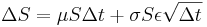
| + | Assume that the drift rate is equal to <math>\mu S</math>, <math>\mu</math> is the expected return of the stock, and variance <math>\sigma^2 S^2</math> and <math>\sigma^2</math> is the variance of the return of the stock. From Weiner process the model for stock prices is: | ||
: <math> \Delta S = \mu S \Delta t + \sigma S \epsilon \sqrt{\Delta t} | : <math> \Delta S = \mu S \Delta t + \sigma S \epsilon \sqrt{\Delta t} | ||
</math> | </math> | ||
Current revision as of 19:04, 3 August 2008
Contents |
SOCR Applications Activities - A Model for Stock Prices
Description
You can access the Stock Prices applet at the SOCR Applications Site, select Financial Applications --> StockSimulation.
Process for Stock Prices
Assume that the drift rate is equal to μS, μ is the expected return of the stock, and variance σ2S2 and σ2 is the variance of the return of the stock. From Weiner process the model for stock prices is:
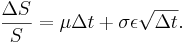
or
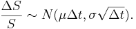
Therefore
- S Price of the stock.
- ΔS Change in the stock price.
- Δt Small interval of time.
- ε Follows N(0,1).
Example
The current price of a stock is  . The expected return is μ = 0.10 per year, and the standard deviation of the return is σ = 0.20 (also per year).
- Find an expression for the process of the stock.
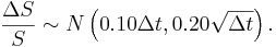
- Find the distribution of the change in S divided by S at the end of the first year. That is, find the distribution of
 .
.
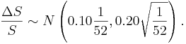
- Divide the year in weekly intervals and find the distribution of at the end of each weekly interval.
- Therefore, sampling from this distribution we can simulate the path of the stock. The price of the stock at the end of the first interval will be S1 = S0 + ΔS1, where ΔS1 is the change during the first time interval, etc.
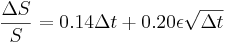
- Using the SOCR applet we will simulate the stock's path by dividing one year into small intervals each one of length
 of a year, when
  , annual mean and standard deviation: μ = 0.14,σ = 0.20.
- The applet will select a random sample of 100 observations from N(0,1) and will compute
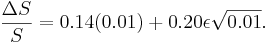
Suppose that ε1 = 0.58. Then

Therefore
- ΔS1 = S0 + ΔS1 = 20 + 0.26 = 20.26.
We continue in the same fashion until we reach the end of the year. Here is the SOCR applet.

- The materials above was partially taken from
Modern Portfolio Theory by Edwin J. Elton, Martin J. Gruber, Stephen J. Brown, and William N. Goetzmann, Sixth Edition, Wiley, 2003, and Options, Futues, and Other Derivatives by John C. Hull, Sixth Edition, Pearson Prentice Hall, 2006.
Translate this page:
