AP Statistics Curriculum 2007 GLM MultLin
From Socr
Contents |
General Advance-Placement (AP) Statistics Curriculum - Multiple Linear Regression
In the previous sections, we saw how to study the relations in bivariate designs. Now we extend that to any finite number of variables (multivariate case).
Multiple Linear Regression
We are interested in determining the linear regression, as a model, of the relationship between one dependent variable Y and many independent variables Xi, i = 1, ..., p. The multilinear regression model can be written as
-
 , where
  is the error term.
The coefficient β0 is the intercept ("constant" term) and βis are the respective parameters of the p independent variables. There are p+1 parameters to be estimated in the multilinear regression.
- Multilinear vs. non-linear regression: This multilinear regression method is "linear" because the relation of the response (the dependent variable Y) to the independent variables is assumed to be a linear function of the parameters βi. Note that multilinear regression is a linear modeling technique not because is that the graph of Y = β0 + βx is a straight line nor because Y is a linear function of the X variables. But the "linear" terms refers to the fact that Y can be considered a linear function of the parameters ( βi), even though it is not a linear function of X. Thus, any model like
-
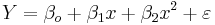
is still one of linear regression, that is, linear in x and x2 respectively, even though the graph on x by itself is not a straight line.
Parameter Estimation in Multilinear Regression
A multilinear regression with p coefficients and the regression intercept β0 and n data points (sample size), with 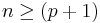 allows construction of the following vectors and matrix with associated standard errors:
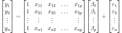
or, in vector-matrix notation
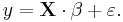
Each data point can be given as  ,
,  . For n = p, standard errors of the parameter estimates could not be calculated. For n less than p, parameters could not be calculated.
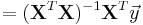
- Point Estimates: The estimated values of the parameters βi are given as

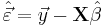
- Residuals: The residuals, representing the difference between the observations and the model's predictions, are required to analyse the regression and are given by:
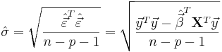
The standard deviation,  for the model is determined from
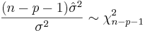
The variance in the errors is Chi-square distributed:
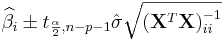
- Interval Estimates: The 100(1 − α)% confidence interval for the parameter, βi, is computed as follows:
 ,
,
where t follows the Student's t-distribution with n − p − 1 degrees of freedom and  denotes the value located in the ith row and column of the matrix.
The regression sum of squares (or sum of squared residuals) SSR (also commonly called RSS) is given by:
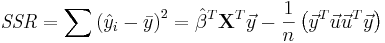 ,
,
where  and
and  is an n by 1 unit vector (i.e. each element is 1). Note that the terms yTu and uTy are both equivalent to
  , and so the term
  is equivalent to
  .
.
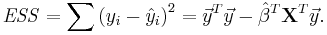
The error (or explained) sum of squares (ESS) is given by:
The total sum of squares (TSS) is given by

Examples
We now demonstrate the use of SOCR Multilinear regression applet to analyze multivariate data.
Earthquake Modeling
This is an example where the relation between variables may not be linear or explanatory. In the simple linear regression case, we were able to compute by hand some (simple) examples. Such calculations are much more involved in the multilinear regression situations. Thus we demonstrate multilinear regression only using the SOCR Multiple Regression Analysis Applet.
Use the SOCR California Earthquake dataset to investigate whether Earthquake magnitude (dependent variable) can be predicted by knowing the longitude, latitude, distance and depth of the quake. Clearly, we do not expect these predictors to have a strong effect on the earthquake magnitude, so we expect the coefficient parameters not to be significantly distinct from zero (null hypothesis). SOCR Multilinear regression applet reports this model:


Multilinear Regression on Consumer Price Index
Using the SOCR Consumer Price Index Dataset we can explore the relationship between the prices of various products and commodities. For example, regressing Gasoline on the following three predictor prices: Orange Juice, Fuel and Electricity illustrates significant effects of all these variables as significant explanatory prices (at α = 0.05) for the cost of Gasoline between 1981 and 2006.


References
- SOCR Home page: http://www.socr.ucla.edu
Translate this page:
