LearningActivities CauchyTGaussian
From Socr
(→Part 1) |
(→Part 1) |
||
| Line 31: | Line 31: | ||
We want the probability that the Pew estimate based on a sample size of <math>n_1=1504</math>, which comes closer to the true value of <math>p</math> than the Opinion Research poll based on <math>n_2=824</math> respondents. | We want the probability that the Pew estimate based on a sample size of <math>n_1=1504</math>, which comes closer to the true value of <math>p</math> than the Opinion Research poll based on <math>n_2=824</math> respondents. | ||
| - | {{hidden|See a Solution to First Part| If <math>\hat{p_1}</math> = the estimate of <math>p</math> from Pew,}} and <math>\hat{p_2}</math> = the estimate of <math>p</math> from Opinion Research, then the problem asks for <math>P[|\hat{p_1}-p| < |\hat{p_1}-p| ]</math>. | + | {{hidden|See a Solution to First Part| test}} |
| + | If <math>\hat{p_1}</math> = the estimate of <math>p</math> from Pew,}} and <math>\hat{p_2}</math> = the estimate of <math>p</math> from Opinion Research, then the problem asks for <math>P[|\hat{p_1}-p| < |\hat{p_1}-p| ]</math>. | ||
: Taking <math>X=\hat{p_1}-p</math> and <math>Y=\hat{p_2}-p</math>, the problem statement indicates that <math>X\sim N(0, \sigma_1^2)</math> and <math>Y\sim N(0, \sigma_2^2)</math>. | : Taking <math>X=\hat{p_1}-p</math> and <math>Y=\hat{p_2}-p</math>, the problem statement indicates that <math>X\sim N(0, \sigma_1^2)</math> and <math>Y\sim N(0, \sigma_2^2)</math>. | ||
Revision as of 20:35, 25 October 2011
Contents |
Distributome Learning Activities - Distributome Activity on the relations between Cauchy, Student's T and Gaussian Distributions
Overview

This activity illustrates the inter-distribution relationships between Cauchy, Student's T and Standard Normal (Gaussian) distributions.
Surveys about public opinions on controversial social issues are becoming increasingly frequent as topics such as the legalization of marijuana, abortion policy, marriage rights for homosexuals, and immigration policy are hotly debated in the media. For example, both the Opinion Research Corporation (polling for CNN) and the Pew Research Center for The People and The Press conducted surveys of American adults in spring of 2011 to estimate the percentage of the public that favors the legalization of marijuana. The sample sizes in the two polls were 824 for the Opinion Research Corporation poll and 1504 for the Pew poll.
Goals
TBD
Hands-on Activity
In this activity you may assume that both of these pollsters use similar techniques that involve telephone interviews and weighting the answers given by individuals to align the respondents demographics with population values and finally averaging to produce unbiased and essentially normally distributed estimates.
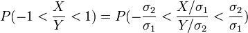
- The Pew poll had almost twice the sample size of the Opinion Research Corporation poll. What is the chance that it was more accurate than that poll for estimating p = the percentage of American adults that favored the legalization of marijuana in spring, 2011? Be sure to clearly define how you are interpreting “more accurate.” Also state and justify any assumptions you make in solving for this probability.
![P[\frac{Accuracy_{poll1}}{Accuracy_{poll2}} < 1]](/distributome/uploads/math/3/f/5/3f550d6b84087a6dbe22468e99f96d70.png) to gauge the chance that one poll s more accurate than the other.
to gauge the chance that one poll s more accurate than the other.
- Describe how you would combine the data from these two polls to form a single estimate of p.
- What is the correlation between your estimate above and the individual estimate produced by the Pew poll?
- What is the probability that your combined estimate from part b) is more accurate than the estimate based only on the Pew poll?
- Note: The questions above may be appropriate for an undergraduate course in probability. The last part would be more appropriate for masters level course (and should have a General Cauchy distribution tag and a tag for its relationship to the bivariate normal).
Solutions
Part 1
We want the probability that the Pew estimate based on a sample size of n1 = 1504, which comes closer to the true value of p than the Opinion Research poll based on n2 = 824 respondents.
If  = the estimate of p from Pew,}} and
  = the estimate of p from Opinion Research, then the problem asks for
 ![P[|\hat{p_1}-p| < |\hat{p_1}-p| ]](/distributome/uploads/math/e/3/3/e332e85bec9f09596964ccdcf50eed32.png) .
.
- Taking
 and
and  , the problem statement indicates that
 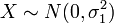 and
and 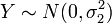 .
.
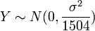
- Also, since the two polls use a similar methodology we may assume that the technique produces estimates with variance
 when a sample size of n is used (for n large enough for the normal approximation to be valid as in these cases).
- Thus,
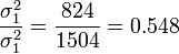 .
.
- Finally, we should assume that the estimates from the two polls are stochastically independent, which is reasonable here since they were conducted by two separate companies and the population of U.S. adults is much larger than either sample size.
- Now
 , where F is the CDF of the Cauchy distribution with scale parameter 0.548 so
 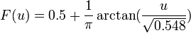 , and the answer is
 ![F(1)-F(-1)=\frac{1}{\pi}[\arctan(\frac{1}{\sqrt{0.548}}) - \arctan(\frac{-1}{\sqrt{0.548}})]\approx 0.594.](/distributome/uploads/math/8/b/0/8b049a98394d0279035545c9d740fad8.png)
- Many people are surprised by how low this answer is - despite having nearly double the sample size, the chance that the Pew poll is more accurate is only 0.594.
- Alternatively, you may solve
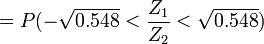 , where Z1 and Z2 are standard normal variables, and their ratio is the standard Cauchy that can then be used to get the correct numerical answer.}}
- Note: A second, more cumbersome, alternative is to work directly to find the marginal distribution of
 from the bivariate normal – see solution to the last part below with ρ = 0.
Part 2
The obvious choice is to propose a linear combination of the two estimates weighting inversely proportional to the variances to get the smallest overall variance amongst such linear combinations:
-
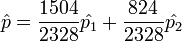 .
.
Of course, this is just the estimate that comes from combining the samples into one large sample of n = 2328 and has variance  .
.
Part 3
Note that  . Thus,
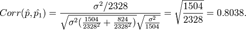 .
.
Part 4
d) We want ![P[|\hat{p}-p| < |\hat{p_1}-p| ]](/distributome/uploads/math/d/6/0/d6072c1a84c630737c2b896f42829ca9.png) .
Taking
.
Taking  and
and  , then
 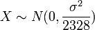 ,
,  and Corr(X,Y) = 0.8038.
Hence,  , where G is the CDF of the generalized Cauchy distribution (see below):
-
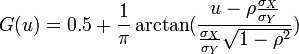 .
.
- So the answer is
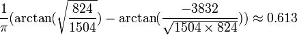 .
.
- So the answer is
Generalized Cauchy distribution CDF derivation
To derive the generalized Cauchy distribution CDF directly, we start with the bivariate normal distribution of X and Y:
-
 .
.
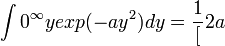
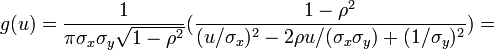
- Then the pdf of
 is:
is:
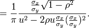
-
 .
.
-
- Since
 , we find that
-
- Thus,
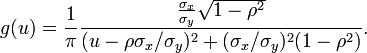
- Finally, we know that
- Thus,
- Therefore, the generalized Cauchy distribution CDF is:
- .
-
Cauchy, Student's T and Gaussian distribution interrelations
The Student's T-distribution represents a one-parameter homotopy path connecting Cauchy and Gaussian Distribution:
-
 .
.
- See the Cauchy, Student's T and Gaussian distribution calculators.
- Explore the relations between these and many other probability distributions using the interactive graphical Distributome Navigator.
Conclusions
TBD
Translate this page:
