LearningActivities ColorBlindness
From Socr
| Line 23: | Line 23: | ||
* Alternatively, to estimate the probability that a randomly selected woman is colorblind, you might use the square of the proportion of colorblind men in a sample of n men. Explain why this estimate makes sense. What is the variance of this estimator? | * Alternatively, to estimate the probability that a randomly selected woman is colorblind, you might use the square of the proportion of colorblind men in a sample of n men. Explain why this estimate makes sense. What is the variance of this estimator? | ||
:: '''Hint''': The moment generating function can be used to find the fourth moment about the origin. | :: '''Hint''': The moment generating function can be used to find the fourth moment about the origin. | ||
| - | :: '''Hint''': We want to estimate <math>p^2</math> and <math>\frac{X_m}{n}</math> estimates <math>p</math> so it makes sense to use <math> | + | :: '''Hint''': We want to estimate <math>p^2</math> and <math>\frac{X_m}{n}</math> estimates <math>p</math> so it makes sense to use <math>(\frac{X_m}{n})^2</math> as the estimator (in fact it will be the [http://wiki.stat.ucla.edu/socr/index.php/AP_Statistics_Curriculum_2007_Estim_MOM_MLE#Maximum_Likelihood_Estimation_.28MLE.29 maximum likelihood estimate]). We have <math>Var[( \frac{X_m}{n} )^2 ] = n^{-4}[E(X_m^4 ) - (E(X_m^2 ))^2 ]</math>. Take <math>q=1-p</math>. Then the fourth moment about the origin of a binomial is <math>E(X^4)= np(q-6pq^2+7npq-11np^2q+6n^2p^2q+n^3p^3)</math> and the second moment is <math>E(X^2)=np(q+np)</math>. Thus <math>Var[( \frac{X_m}{n} )^2 ] = n^{-3}(pq + 6(n-1)p^2q^2 + 4n(n-1)p^3q)</math>. |
# For large samples, is it better to use a sample of men or a sample of women to estimate the probability that a randomly selected women is colorblind? Explain. | # For large samples, is it better to use a sample of men or a sample of women to estimate the probability that a randomly selected women is colorblind? Explain. | ||
| + | :: '''Hint''': Show that a normal approximation is valid for both and then compare the variances. | ||
| - | + | ::'''Solution''': For large n the ratio of the variances for the estimate in part c to the estimate in part d is <math>\frac{Var(\frac{X_f}{n})}{Var((\frac{X_m}{n})^2 )} \sim \frac{p^2(1-p^2)}{4p^3q} = \frac{1+ p}{4p}</math>. When this ratio is greater than 1, the estimator based on the sample of men will be better. Since this happens for any <math>p\lt \frac{1}{3}</math>, which is clearly the case for colorblindness, it is better to use a sample of men to estimate the probability that a random woman is colorblind. | |
| - | + | ||
| - | '''Solution''': For large n the ratio of the variances for the estimate in part c to the estimate in part d is Var( | + | |
===Conclusions=== | ===Conclusions=== | ||
You can also use the delta method to find the approximate variance for the estimator above. | You can also use the delta method to find the approximate variance for the estimator above. | ||
| - | |||
{{translate|pageName=http://wiki.stat.ucla.edu/distributome/index.php?title=LearningActivities_ColorBlindness}} | {{translate|pageName=http://wiki.stat.ucla.edu/distributome/index.php?title=LearningActivities_ColorBlindness}} | ||
Revision as of 00:03, 25 October 2011
Contents |
Distributome Learning Activities - Distributome Colorblindness Activity
Overview
This Distributome Activity illustrates an application of probability theory to study Colorblindness.
Colorblindness results from an abnormality on the X chromosome. The condition is thus rarer in women since a woman would need to have the abnormality on both of her X chromosomes in order to be colorblind (whether a woman has the abnormality on one X chromosome is essentially independent of having it on the other).
Goals
The goal of this activity is to demonstrate an efficient protocol of estimating the probability that a randomly chosen individual may be colorblind.
Hands-on Activity
Suppose that p is the probability that a randomly selected man is colorblind.
- 100 men are selected at random. What is the distribution of Xm = the number of these men that are colorblind?
- Xm~Binomial(100,p).
- 100 women are selected at random. What is the distribution of Xf = the number of these women that are colorblind?
- Hint: the chance that an individual woman is colorblind is p2, why?
- Solution: Xf~Binomial(100,p2)
- To estimate the probability that a randomly selected woman is colorblind, you might use the proportion of colorblind women in a sample of n women. What is the variance of this estimator?
- Xf~Binomial(n,p2). Thus
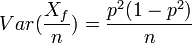 .
.
- Xf~Binomial(n,p2). Thus
- Alternatively, to estimate the probability that a randomly selected woman is colorblind, you might use the square of the proportion of colorblind men in a sample of n men. Explain why this estimate makes sense. What is the variance of this estimator?
- Hint: The moment generating function can be used to find the fourth moment about the origin.
- Hint: We want to estimate p2 and
 estimates p so it makes sense to use
  as the estimator (in fact it will be the maximum likelihood estimate). We have
 ![Var[( \frac{X_m}{n} )^2 ] = n^{-4}[E(X_m^4 ) - (E(X_m^2 ))^2 ]](/distributome/uploads/math/7/b/1/7b1d064eb834c54f5fa75fccf0b68fa6.png) . Take q = 1 − p. Then the fourth moment about the origin of a binomial is E(X4) = np(q − 6pq2 + 7npq − 11np2q + 6n2p2q + n3p3) and the second moment is E(X2) = np(q + np). Thus
. Take q = 1 − p. Then the fourth moment about the origin of a binomial is E(X4) = np(q − 6pq2 + 7npq − 11np2q + 6n2p2q + n3p3) and the second moment is E(X2) = np(q + np). Thus ![Var[( \frac{X_m}{n} )^2 ] = n^{-3}(pq + 6(n-1)p^2q^2 + 4n(n-1)p^3q)](/distributome/uploads/math/a/7/5/a758430bad27ccec1ecba7e928df8764.png) .
.
- For large samples, is it better to use a sample of men or a sample of women to estimate the probability that a randomly selected women is colorblind? Explain.
- Hint: Show that a normal approximation is valid for both and then compare the variances.
- Solution: For large n the ratio of the variances for the estimate in part c to the estimate in part d is
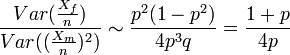 . When this ratio is greater than 1, the estimator based on the sample of men will be better. Since this happens for any Failed to parse (unknown function\lt): p\lt \frac{1}{3}
- Solution: For large n the ratio of the variances for the estimate in part c to the estimate in part d is
, which is clearly the case for colorblindness, it is better to use a sample of men to estimate the probability that a random woman is colorblind.
Conclusions
You can also use the delta method to find the approximate variance for the estimator above.
Translate this page:
