AP Statistics Curriculum 2007 Gamma
From Socr
(→Gamma Distribution) |
m (→Normal Approximation to Gamma distribution) |
||
| (31 intermediate revisions not shown) | |||
| Line 1: | Line 1: | ||
| - | === Gamma Distribution === | + | ==[[AP_Statistics_Curriculum_2007 | General Advance-Placement (AP) Statistics Curriculum]] - Gamma Distribution== |
| + | |||
| + | ===Gamma Distribution=== | ||
'''Definition''': Gamma distribution is a distribution that arises naturally in processes for which the waiting times between events are relevant. It can be thought of as a waiting time between Poisson distributed events. | '''Definition''': Gamma distribution is a distribution that arises naturally in processes for which the waiting times between events are relevant. It can be thought of as a waiting time between Poisson distributed events. | ||
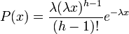
| - | <br />'''Probability density function''': The waiting time until the hth Poisson event with a rate of change <math>\lambda</math> is | + | <br />'''Probability density function''': The waiting time until the hth Poisson event with a rate of change <font size="3"><math>\lambda</math></font> is |
:<math>P(x)=\frac{\lambda(\lambda x)^{h-1}}{(h-1)!}{e^{-\lambda x}}</math> | :<math>P(x)=\frac{\lambda(\lambda x)^{h-1}}{(h-1)!}{e^{-\lambda x}}</math> | ||
| - | For X | + | For <math>X\sim \operatorname{Gamma}(k,\theta)\!</math>, where <font size="3"><math>k=h</math></font> and <font size="3"><math>\theta=1/\lambda</math></font>, the gamma probability density function is given by |
:<math>\frac{x^{k-1}e^{-x/\theta}}{\Gamma(k)\theta^k}</math> | :<math>\frac{x^{k-1}e^{-x/\theta}}{\Gamma(k)\theta^k}</math> | ||
| Line 14: | Line 16: | ||
*e is the natural number (e = 2.71828…) | *e is the natural number (e = 2.71828…) | ||
*k is the number of occurrences of an event | *k is the number of occurrences of an event | ||
| - | *if k is a positive integer, then <math>\Gamma(k)=(k-1)!</math> is the gamma function | + | *if k is a positive integer, then <font size="3"><math>\Gamma(k)=(k-1)!</math></font> is the gamma function |
| - | *<math>\theta=1/\lambda</math> is the mean number of events per time unit, where <math>\lambda</math> is the mean time between events. For example, if the mean time between phone calls is 2 hours, then you would use a gamma distribution with <math>\theta</math>=1/2=0.5. If we want to find the mean number of calls in 5 hours, it would be 5 <math>\times</math> 1/2=2.5. | + | *<font size="3"><math>\theta=1/\lambda</math></font> is the mean number of events per time unit, where <font size="3"><math>\lambda</math></font> is the mean time between events. For example, if the mean time between phone calls is 2 hours, then you would use a gamma distribution with <font size="3"><math>\theta</math>=1/2=0.5</font>. If we want to find the mean number of calls in 5 hours, it would be <font size="3">5 <math>\times</math> 1/2=2.5</font>. |
*x is a random variable | *x is a random variable | ||
| Line 23: | Line 25: | ||
where | where | ||
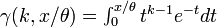
| - | *if k is a positive integer, then <math>\Gamma(k)=(k-1)!</math> is the gamma function | + | *if k is a positive integer, then <font size="3"><math>\Gamma(k)=(k-1)!</math></font> is the gamma function |
| - | *<math>\gamma(k,x/\theta)=\int_0^{x/\theta}t^{k-1}e^{-t}dt</math> | + | *<math>\textstyle\gamma(k,x/\theta)=\int_0^{x/\theta}t^{k-1}e^{-t}dt</math> |
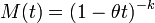
<br />'''Moment generating function''': The gamma moment-generating function is | <br />'''Moment generating function''': The gamma moment-generating function is | ||
| Line 47: | Line 49: | ||
The gamma distribution is also used to model errors in a multi-level Poisson regression model because the combination of a Poisson distribution and a gamma distribution is a negative binomial distribution. | The gamma distribution is also used to model errors in a multi-level Poisson regression model because the combination of a Poisson distribution and a gamma distribution is a negative binomial distribution. | ||
| - | |||
===Example=== | ===Example=== | ||
Suppose you are fishing and you expect to get a fish once every 1/2 hour. Compute the probability that you will have to wait between 2 to 4 hours before you catch 4 fish. | Suppose you are fishing and you expect to get a fish once every 1/2 hour. Compute the probability that you will have to wait between 2 to 4 hours before you catch 4 fish. | ||
| - | One fish every 1/2 hour means we would expect to get <math>\theta=1/0.5=2</math> fish every hour on average. Using <math>\theta=2</math> and <math>k=4</math>, we can compute this as follows: | + | One fish every 1/2 hour means we would expect to get <font size="3"><math>\theta=1 / 0.5=2</math></font> fish every hour on average. Using <font size="3"><math>\theta=2</math></font> and <font size="3"><math>k=4</math></font>, we can compute this as follows: |
| + | |||
:<math>P(2\le X\le 4)=\sum_{x=2}^4\frac{x^{4-1}e^{-x/2}}{\Gamma(4)2^4}=0.12388</math> | :<math>P(2\le X\le 4)=\sum_{x=2}^4\frac{x^{4-1}e^{-x/2}}{\Gamma(4)2^4}=0.12388</math> | ||
The figure below shows this result using [http://socr.ucla.edu/htmls/dist/Gamma_Distribution.html SOCR distributions] | The figure below shows this result using [http://socr.ucla.edu/htmls/dist/Gamma_Distribution.html SOCR distributions] | ||
<center>[[Image:Gamma.jpg|600px]]</center> | <center>[[Image:Gamma.jpg|600px]]</center> | ||
| + | |||
| + | |||
| + | ===Normal Approximation to Gamma distribution=== | ||
| + | |||
| + | Note that if \( \{X_1,X_2,X_3,\cdots \}\) is a sequence of independent [[AP_Statistics_Curriculum_2007_Exponential|Exponential(b) random variables]] then \(Y_k = \sum_{i=1}^k{X_i} \) is a [http://www.math.uah.edu/stat/special/Gamma.html random variable with gamma distribution] with the following shape parameter, '''k''' (positive integer indicating the number of exponential variable in the sum) and scale parameter '''b''' (which is the exponential parameter). By the [[AP_Statistics_Curriculum_2007_Limits_CLT|central limit theorem]], if k is large, then gamma distribution can be approximated by the normal distribution with mean \(\mu=kb\) and variance \(\sigma^2 =kb^2\). That is, the distribution of the variable \(Z_k={{Y_k-kb}\over{\sqrt{k}b}}\) tends to the standard normal distribution as <math>k\longrightarrow \infty</math>. | ||
| + | |||
| + | For the example above, \(\Gamma(k=4, \theta=2)\), the [http://socr.ucla.edu/htmls/dist/Gamma_Distribution.html SOCR Normal Distribution Calculator] can be used to obtain an estimate of the area of interest as shown on the image below. | ||
| + | |||
| + | <center>[[Image:EBook_Gamma_Fig2.png|500px]]</center> | ||
| + | |||
| + | The probabilities of the [http://socr.ucla.edu/htmls/dist/Gamma_Distribution.html real Gamma] and [http://socr.ucla.edu/htmls/dist/Normal_Distribution.html approximate Normal] distributions (on the range [2:4]) are not identical but are sufficiently close. | ||
| + | |||
| + | <center> | ||
| + | {| class="wikitable" style="text-align:center; width:75%" border="1" | ||
| + | |- | ||
| + | ! Summary|| [http://socr.ucla.edu/htmls/dist/Gamma_Distribution.html \(\Gamma(k=4, \theta=2)\) ] || [http://socr.ucla.edu/htmls/dist/Normal_Distribution.html \(Normal(\mu=8, \sigma^2=4)\) ] | ||
| + | |- | ||
| + | | Mean||8.000000||8.0 | ||
| + | |- | ||
| + | | Median||7.32||8.0 | ||
| + | |- | ||
| + | | Variance||16.0||16.0 | ||
| + | |- | ||
| + | | Standard Deviation||4.0||4.0 | ||
| + | |- | ||
| + | | Max Density|| 0.112021||0.099736 | ||
| + | |- | ||
| + | ! colspan=3|Probability Areas | ||
| + | |- | ||
| + | | <2|| 0.018988|| 0.066807 | ||
| + | |- | ||
| + | | [2:4]|| 0.123888||0.091848 | ||
| + | |- | ||
| + | | >4|| 0.857123||0.841345 | ||
| + | |} | ||
| + | </center> | ||
| + | |||
| + | <hr> | ||
| + | * SOCR Home page: http://www.socr.ucla.edu | ||
| + | |||
| + | {{translate|pageName=http://wiki.stat.ucla.edu/socr/index.php/AP_Statistics_Curriculum_2007_Gamma}} | ||
Current revision as of 17:34, 23 June 2012
Contents |
General Advance-Placement (AP) Statistics Curriculum - Gamma Distribution
Gamma Distribution
Definition: Gamma distribution is a distribution that arises naturally in processes for which the waiting times between events are relevant. It can be thought of as a waiting time between Poisson distributed events.
Probability density function: The waiting time until the hth Poisson event with a rate of change λ is
For 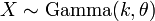 , where k = h and θ = 1 / λ, the gamma probability density function is given by

where
- e is the natural number (e = 2.71828…)
- k is the number of occurrences of an event
- if k is a positive integer, then Γ(k) = (k − 1)! is the gamma function
- θ = 1 / λ is the mean number of events per time unit, where λ is the mean time between events. For example, if the mean time between phone calls is 2 hours, then you would use a gamma distribution with θ=1/2=0.5. If we want to find the mean number of calls in 5 hours, it would be 5
 1/2=2.5.
- x is a random variable
Cumulative density function: The gamma cumulative distribution function is given by

where
- if k is a positive integer, then Γ(k) = (k − 1)! is the gamma function
Moment generating function: The gamma moment-generating function is
Expectation: The expected value of a gamma distributed random variable x is

Variance: The gamma variance is
Applications
The gamma distribution can be used a range of disciplines including queuing models, climatology, and financial services. Examples of events that may be modeled by gamma distribution include:
- The amount of rainfall accumulated in a reservoir
- The size of loan defaults or aggregate insurance claims
- The flow of items through manufacturing and distribution processes
- The load on web servers
- The many and varied forms of telecom exchange
The gamma distribution is also used to model errors in a multi-level Poisson regression model because the combination of a Poisson distribution and a gamma distribution is a negative binomial distribution.
Example
Suppose you are fishing and you expect to get a fish once every 1/2 hour. Compute the probability that you will have to wait between 2 to 4 hours before you catch 4 fish.
One fish every 1/2 hour means we would expect to get θ = 1 / 0.5 = 2 fish every hour on average. Using θ = 2 and k = 4, we can compute this as follows:
The figure below shows this result using SOCR distributions

Normal Approximation to Gamma distribution
Note that if \( \{X_1,X_2,X_3,\cdots \}\) is a sequence of independent Exponential(b) random variables then \(Y_k = \sum_{i=1}^k{X_i} \) is a random variable with gamma distribution with the following shape parameter, k (positive integer indicating the number of exponential variable in the sum) and scale parameter b (which is the exponential parameter). By the central limit theorem, if k is large, then gamma distribution can be approximated by the normal distribution with mean \(\mu=kb\) and variance \(\sigma^2 =kb^2\). That is, the distribution of the variable \(Z_k={{Y_k-kb}\over{\sqrt{k}b}}\) tends to the standard normal distribution as  .
.
For the example above, \(\Gamma(k=4, \theta=2)\), the SOCR Normal Distribution Calculator can be used to obtain an estimate of the area of interest as shown on the image below.

The probabilities of the real Gamma and approximate Normal distributions (on the range [2:4]) are not identical but are sufficiently close.
| Summary | \(\Gamma(k=4, \theta=2)\) | \(Normal(\mu=8, \sigma^2=4)\) |
|---|---|---|
| Mean | 8.000000 | 8.0 |
| Median | 7.32 | 8.0 |
| Variance | 16.0 | 16.0 |
| Standard Deviation | 4.0 | 4.0 |
| Max Density | 0.112021 | 0.099736 |
| Probability Areas | ||
| <2 | 0.018988 | 0.066807 |
| [2:4] | 0.123888 | 0.091848 |
| >4 | 0.857123 | 0.841345 |
- SOCR Home page: http://www.socr.ucla.edu
Translate this page:
