AP Statistics Curriculum 2007 Fisher F
From Socr
(Created page with '== General Advance-Placement (AP) Statistics Curriculum - Fisher's F Distribution== ===Fisher's F Distribution=== Commonly used as the null di…') |
|||
| Line 24: | Line 24: | ||
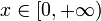
<math>x \in [0, +\infty)\!</math> | <math>x \in [0, +\infty)\!</math> | ||
| - | + | ===Applications=== | |
| + | [http://en.wikipedia.org/wiki/ANOVA ANOVA] | ||
| + | ===Example=== | ||
| + | We want to examine the effect of three different brands of gasoline on gas mileage using an alpha value of 0.05. We will have 6 observations for each of the 3 gasoline brands. Gas mileage figures are as follows: | ||
| - | + | {| class="wikitable" | |
| + | |- | ||
| + | ! Brand A | ||
| + | ! Brand B | ||
| + | ! Brand C | ||
| + | |- | ||
| + | | 29 | ||
| + | | 30 | ||
| + | | 28 | ||
| + | |- | ||
| + | | 30 | ||
| + | | 31 | ||
| + | | 29 | ||
| + | |- | ||
| + | | 29 | ||
| + | | 32 | ||
| + | | 28 | ||
| + | |- | ||
| + | | 28 | ||
| + | | 29 | ||
| + | | 26 | ||
| + | |- | ||
| + | | 30 | ||
| + | | 31 | ||
| + | | 30 | ||
| + | |- | ||
| + | | 28 | ||
| + | | 33 | ||
| + | | 29 | ||
| + | |} | ||
| + | Our null hypothesis, <math>H_0</math>, is that the three brands of gasoline will yield the same amount of gas mileage, on average. | ||
| - | ''' | + | First, we find the F-ratio: |
| + | |||
| + | '''Step 1:''' Calculate the mean for each brand: <br> | ||
| + | |||
| + | Brand A: <math>\overline{Y}_1=\tfrac{29+30+29+28+30+28}{6} = 29</math> | ||
| + | |||
| + | Brand B: <math>\overline{Y}_2\tfrac{30+31+32+29+31+33}{6} = 31</math> | ||
| + | |||
| + | Brand C: <math>\overline{Y}_3\tfrac{28+29+28+26+30+29}{6} = 28</math> | ||
| + | |||
| + | |||
| + | '''Step 2:''' Calculate the overall mean: <br> | ||
| + | |||
| + | ===<math>\overline{Y}=29+31+28=29.67</math>=== | ||
| + | |||
| + | '''Step 3:''' Calculate the Between-Group Sum of Squares: <br> | ||
| + | |||
| + | <math> | ||
| + | \begin{align} | ||
| + | SS_b &= n(\overline{Y}_1-\overline{Y})^2+n(\overline{Y}_2-\overline{Y})^2+n(\overline{Y}_3-\overline{Y})^2\\ | ||
| + | &= 6(29-29.67)^2+6(31-29.67)^2+6(28-29.67)^2=30.04 | ||
| + | \end{align} | ||
| + | </math> | ||
| + | |||
| + | Where n is the number of observations per group. | ||
| + | |||
| + | The between-group degrees of freedom is one less than the number of groups: 3-1=2. | ||
| + | |||
| + | Therefore, the between-group mean square value, <math>MS_B</math>, is <math>\tfrac{30.04}{2}=15.02</math> | ||
| + | |||
| + | '''Step 4:''' Calculate the Within-Group Sum of Squares: <br> | ||
| + | |||
| + | We start by subtracting each observation by its group mean: | ||
| + | |||
| + | {| class="wikitable" | ||
| + | |- | ||
| + | ! Brand A | ||
| + | ! Brand B | ||
| + | ! Brand C | ||
| + | |- | ||
| + | | 29-29=0 | ||
| + | | 30-31=-1 | ||
| + | | 28-28=0 | ||
| + | |- | ||
| + | | 30-29=1 | ||
| + | | 31-31=0 | ||
| + | | 29-28=1 | ||
| + | |- | ||
| + | | 29-29=0 | ||
| + | | 32-31=1 | ||
| + | | 28-28=0 | ||
| + | |- | ||
| + | | 28-29=-1 | ||
| + | | 29-31=-2 | ||
| + | | 26-28=-2 | ||
| + | |- | ||
| + | | 30-29=1 | ||
| + | | 31-31=0 | ||
| + | | 30-28=2 | ||
| + | |- | ||
| + | | 28-29=-1 | ||
| + | | 33-31=2 | ||
| + | | 29-28=1 | ||
| + | |} | ||
| + | |||
| + | The Within-Group Sum of Squares, <math>SS_w</math>, is the sum of the squares of the values in the previous table: | ||
| + | |||
| + | <math>0+1+0+1+0+1+0+1+0+1+4+4+1+0+4+1+4+1=24</math> | ||
| + | |||
| + | The Within-Group degrees of freedom is the number of groups times 1 less the number of observations per group: | ||
| + | |||
| + | <math>3(6-1)=15</math> | ||
| + | |||
| + | The Within-Group Mean Square Value, <math>MS_W</math> is: <math>\tfrac{24}{15}=1.6</math> | ||
| + | |||
| + | '''Step 5:''' Finally, the F-Ratio is: | ||
| + | |||
| + | <math>\tfrac{MS_B}{MS_W}=\tfrac{15.02}{1.6}=9.39</math> | ||
| + | |||
| + | The F critical value is the value that the test statistic must exceed in order to reject the <math>H_0</math>. In this case, <math>F_crit(2,15)=3.68</math> at <math>\alpha=0.05</math>. Since F=9.39>3.68, we reject <math>H_0</math> at the 5% significance level, concluding that there is a difference in gas mileage between the gasoline brands. | ||
| + | |||
| + | We can find the critical F-value using the SOCR F Distribution Calculator: | ||
| + | |||
| + | [[File:F.png]] | ||
| + | |||
| + | ===SOCR Links=== | ||
| + | http://www.distributome.org/ -> SOCR -> Distributions -> Fisher’s F | ||
| + | |||
| + | http://www.distributome.org/ -> SOCR -> Distributions -> Fisher’s F Distribution | ||
| + | |||
| + | http://www.distributome.org/ -> SOCR -> Functors -> Fisher’s F Distribution | ||
| + | |||
| + | http://www.distributome.org/ -> SOCR -> Analyses -> ANOVA – One Way | ||
| + | |||
| + | http://www.distributome.org/ -> SOCR -> Analyses -> ANOVA – Two Way | ||
| + | |||
| + | SOCR F-Distribution Calculator (http://socr.ucla.edu/htmls/dist/Fisher_Distribution.html) | ||
Revision as of 06:14, 3 July 2011
Contents |
General Advance-Placement (AP) Statistics Curriculum - Fisher's F Distribution
Fisher's F Distribution
Commonly used as the null distribution of a test statistic, such as in analysis of variance (ANOVA). Relationship to the t-distribution and [beta Distribution].
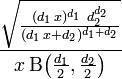
PDF:
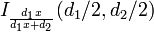
CDF:
Mean:
 for d2 > 2
Median:
None
Variance:
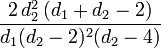 for d2 > 4
Support:
Applications
Example
We want to examine the effect of three different brands of gasoline on gas mileage using an alpha value of 0.05. We will have 6 observations for each of the 3 gasoline brands. Gas mileage figures are as follows:
| Brand A | Brand B | Brand C |
|---|---|---|
| 29 | 30 | 28 |
| 30 | 31 | 29 |
| 29 | 32 | 28 |
| 28 | 29 | 26 |
| 30 | 31 | 30 |
| 28 | 33 | 29 |
Our null hypothesis, H0, is that the three brands of gasoline will yield the same amount of gas mileage, on average.
First, we find the F-ratio:
Step 1: Calculate the mean for each brand:
Brand A: 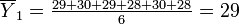
Brand B: 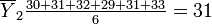
Brand C: 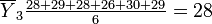
Step 2: Calculate the overall mean:

Step 3: Calculate the Between-Group Sum of Squares:

Where n is the number of observations per group.
The between-group degrees of freedom is one less than the number of groups: 3-1=2.
Therefore, the between-group mean square value, MSB, is 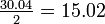
Step 4: Calculate the Within-Group Sum of Squares:
We start by subtracting each observation by its group mean:
| Brand A | Brand B | Brand C |
|---|---|---|
| 29-29=0 | 30-31=-1 | 28-28=0 |
| 30-29=1 | 31-31=0 | 29-28=1 |
| 29-29=0 | 32-31=1 | 28-28=0 |
| 28-29=-1 | 29-31=-2 | 26-28=-2 |
| 30-29=1 | 31-31=0 | 30-28=2 |
| 28-29=-1 | 33-31=2 | 29-28=1 |
The Within-Group Sum of Squares, SSw, is the sum of the squares of the values in the previous table:
0 + 1 + 0 + 1 + 0 + 1 + 0 + 1 + 0 + 1 + 4 + 4 + 1 + 0 + 4 + 1 + 4 + 1 = 24
The Within-Group degrees of freedom is the number of groups times 1 less the number of observations per group:
3(6 − 1) = 15
The Within-Group Mean Square Value, MSW is: 
Step 5: Finally, the F-Ratio is:
The F critical value is the value that the test statistic must exceed in order to reject the H0. In this case, Fcrit(2,15) = 3.68 at α = 0.05. Since F=9.39>3.68, we reject H0 at the 5% significance level, concluding that there is a difference in gas mileage between the gasoline brands.
We can find the critical F-value using the SOCR F Distribution Calculator:

SOCR Links
http://www.distributome.org/ -> SOCR -> Distributions -> Fisher’s F
http://www.distributome.org/ -> SOCR -> Distributions -> Fisher’s F Distribution
http://www.distributome.org/ -> SOCR -> Functors -> Fisher’s F Distribution
http://www.distributome.org/ -> SOCR -> Analyses -> ANOVA – One Way
http://www.distributome.org/ -> SOCR -> Analyses -> ANOVA – Two Way
SOCR F-Distribution Calculator (http://socr.ucla.edu/htmls/dist/Fisher_Distribution.html)
