AP Statistics Curriculum 2007 Gamma
From Socr
(added Normal approximation to Gamma) |
|||
| Line 59: | Line 59: | ||
The figure below shows this result using [http://socr.ucla.edu/htmls/dist/Gamma_Distribution.html SOCR distributions] | The figure below shows this result using [http://socr.ucla.edu/htmls/dist/Gamma_Distribution.html SOCR distributions] | ||
<center>[[Image:Gamma.jpg|600px]]</center> | <center>[[Image:Gamma.jpg|600px]]</center> | ||
| + | |||
| + | |||
| + | ===Normal Approximation to Gamma distribution=== | ||
| + | |||
| + | Note that if \( \{X_1,X_2,X_3,\cdots \}\) is a sequence of independent [[AP_Statistics_Curriculum_2007_Exponential|Exponential random variables]] then \(Y_k = \sum_{i=1}^k{X_i} \) is a [http://www.math.uah.edu/stat/special/Gamma.html random variable with gamma distribution with some shape parameter], k (positive integer) and scale parameter b. By the [[AP_Statistics_Curriculum_2007_Limits_CLT|central limit theorem]], if k is large, then gamma distribution can be approximated by the normal distribution with mean \(\mu=kb\) and variance \(\sigma =kb^2\). That is, the distribution of the variable <math>Z_k=\fract{Y_k-kb}{\sqrt{k}b}</math> tends to the standard normal distribution as <math>k\longrightarrow \infty</math>. | ||
<hr> | <hr> | ||
Revision as of 16:55, 23 June 2012
Contents |
General Advance-Placement (AP) Statistics Curriculum - Gamma Distribution
Gamma Distribution
Definition: Gamma distribution is a distribution that arises naturally in processes for which the waiting times between events are relevant. It can be thought of as a waiting time between Poisson distributed events.
Probability density function: The waiting time until the hth Poisson event with a rate of change λ is
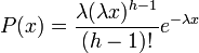
For  , where k = h and θ = 1 / λ, the gamma probability density function is given by

where
- e is the natural number (e = 2.71828…)
- k is the number of occurrences of an event
- if k is a positive integer, then Γ(k) = (k − 1)! is the gamma function
- θ = 1 / λ is the mean number of events per time unit, where λ is the mean time between events. For example, if the mean time between phone calls is 2 hours, then you would use a gamma distribution with θ=1/2=0.5. If we want to find the mean number of calls in 5 hours, it would be 5
 1/2=2.5.
- x is a random variable
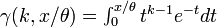
Cumulative density function: The gamma cumulative distribution function is given by

where
- if k is a positive integer, then Γ(k) = (k − 1)! is the gamma function
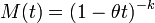
Moment generating function: The gamma moment-generating function is
Expectation: The expected value of a gamma distributed random variable x is

Variance: The gamma variance is
Applications
The gamma distribution can be used a range of disciplines including queuing models, climatology, and financial services. Examples of events that may be modeled by gamma distribution include:
- The amount of rainfall accumulated in a reservoir
- The size of loan defaults or aggregate insurance claims
- The flow of items through manufacturing and distribution processes
- The load on web servers
- The many and varied forms of telecom exchange
The gamma distribution is also used to model errors in a multi-level Poisson regression model because the combination of a Poisson distribution and a gamma distribution is a negative binomial distribution.
Example
Suppose you are fishing and you expect to get a fish once every 1/2 hour. Compute the probability that you will have to wait between 2 to 4 hours before you catch 4 fish.
One fish every 1/2 hour means we would expect to get θ = 1 / 0.5 = 2 fish every hour on average. Using θ = 2 and k = 4, we can compute this as follows:
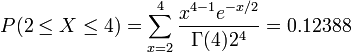
The figure below shows this result using SOCR distributions

Normal Approximation to Gamma distribution
Note that if \( \{X_1,X_2,X_3,\cdots \}\) is a sequence of independent Exponential random variables then \(Y_k = \sum_{i=1}^k{X_i} \) is a random variable with gamma distribution with some shape parameter, k (positive integer) and scale parameter b. By the central limit theorem, if k is large, then gamma distribution can be approximated by the normal distribution with mean \(\mu=kb\) and variance \(\sigma =kb^2\). That is, the distribution of the variable Failed to parse (unknown function\fract): Z_k=\fract{Y_k-kb}{\sqrt{k}b}
tends to the standard normal distribution as.
- SOCR Home page: http://www.socr.ucla.edu
Translate this page:
