SOCR EduMaterials Activities ApplicationsActivities Portfolio
From Socr
Portfolio Theory
An investor has a certain amount of dollars to invest into two stocks
(IBM and TEXACO). A portion of the available funds will be invested into
IBM (denote this portion of the funds with xA) and the remaining funds
into TEXACO (denote it with xB) - so xA + xB = 1. The resulting portfolio
will be xARA + xBRB, where RA is the monthly return of IBM and RB is the
monthly return of TEXACO. The goal here is to
find the most efficient portfolios given a certain amount of risk.
Using market data from January 1980 until February 2001 we compute
that E(RA) = 0.010, E(RB) = 0.013, Var(RA) = 0.0061, Var(RB) = 0.0046, and
Cov(RA,RB) = 0.00062. We first want to minimize the variance of the portfolio.
This will be:
 Or
Or

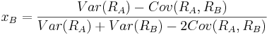
Therefore our goal is to find xA and xB, the percentage of the
available funds that will be invested in each stock. Substituting
xB = 1 − xA into the equation of the variance we get

To minimize the above exression we take the derivative with respect to
xA, set it equal to zero and solve for xA. The result is:
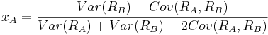 and therefore
 The values of xa and xB are:
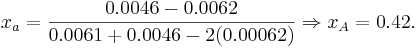 and
and  . Therefore if the investor invests
 of the available funds into IBM and the remaining
  into TEXACO the variance of the portfolio will be minimum and equal to:
Var(0.42RA + 0.58RB) = 0.422(0.0061) + 0.582(0.0046) + 2(0.42)(0.58)(0.00062) = 0.002926.
The corresponding expected return of this porfolio will be:
E(0.42RA + 0.58RB) = 0.42(0.010) + 0.58(0.013) = 0.01174.
We can try many other combinations of xA and xB (but always xA + xB = 1)
and compute the risk and return for each resulting portfolio. This is
shown in the table and the graph below.
into TEXACO the variance of the portfolio will be minimum and equal to:
Var(0.42RA + 0.58RB) = 0.422(0.0061) + 0.582(0.0046) + 2(0.42)(0.58)(0.00062) = 0.002926.
The corresponding expected return of this porfolio will be:
E(0.42RA + 0.58RB) = 0.42(0.010) + 0.58(0.013) = 0.01174.
We can try many other combinations of xA and xB (but always xA + xB = 1)
and compute the risk and return for each resulting portfolio. This is
shown in the table and the graph below.
| xA | xB | Risk (σ2) | Return | Risk (σ) |
|---|---|---|---|---|
| 1.00 | 0.00 | 0.006100 | 0.01000 | 0.078102 |
| 0.95 | 0.05 | 0.005576 | 0.01015 | 0.074670 |
| 0.90 | 0.10 | 0.005099 | 0.01030 | 0.071404 |
| 0.85 | 0.15 | 0.004669 | 0.01045 | 0.068329 |
| 0.80 | 0.20 | 0.004286 | 0.01060 | 0.065471 |
| 0.75 | 0.25 | 0.003951 | 0.01075 | 0.062859 |
| 0.70 | 0.30 | 0.003663 | 0.01090 | 0.060526 |
| 0.65 | 0.35 | 0.003423 | 0.01105 | 0.058505 |
| 0.60 | 0.40 | 0.003230 | 0.01120 | 0.056830 |
| 0.55 | 0.45 | 0.003084 | 0.01135 | 0.055531 |
| 0.50 | 0.50 | 0.002985 | 0.01150 | 0.054635 |
| 0.42 | 0.58 | 0.002926 | 0.01174 | 0.054088 |
| 0.40 | 0.60 | 0.002930 | 0.01180 | 0.054126 |
| 0.35 | 0.65 | 0.002973 | 0.01195 | 0.054524 |
| 0.30 | 0.70 | 0.003063 | 0.01210 | 0.055348 |
| 0.25 | 0.75 | 0.003201 | 0.01225 | 0.056580 |
| 0.20 | 0.80 | 0.003386 | 0.01240 | 0.058193 |
| 0.15 | 0.85 | 0.003619 | 0.01255 | 0.060157 |
| 0.10 | 0.90 | 0.003899 | 0.01270 | 0.062439 |
| 0.05 | 0.95 | 0.004226 | 0.01285 | 0.065005 |
| 0.00 | 1.00 | 0.004600 | 0.01300 | 0.067823 |
For the above calculations short selling was not allowed ( and
and
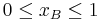 , in addition to xA + xB = 1). We note here that the efficient portfolios are located on the top part of the graph between the minimum risk portfolio point and the maximum return portfolio point, which is called the efficient frontier (the blue portion of the graph). Efficient portfolios should provide higher expected return for the same level of risk or lower risk for the same level of expected return.
