AP Statistics Curriculum 2007 Bayesian Prelim
From Socr
| Line 13: | Line 13: | ||
What is commonly called '''Bayesian Statistics''' is a very special application of Bayes Theorem. | What is commonly called '''Bayesian Statistics''' is a very special application of Bayes Theorem. | ||
| - | We will examine a number of examples in this Chapter, but to illustrate generally, imagine that '''x''' is a fixed collection of data that has been realized from under some known density, <math>f(\cdot)</math> that takes a parameter, <math>\mu</math> whose value is not certainly known. | + | We will examine a number of examples in this Chapter, but to illustrate generally, imagine that '''x''' is a fixed collection of data that has been realized from under some known density, <math>f(\cdot)</math>, that takes a parameter, <math>\mu</math>, whose value is not certainly known. |
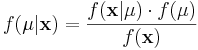
Using Bayes Theorem we may write | Using Bayes Theorem we may write | ||
| Line 19: | Line 19: | ||
<math>f(\mu|\mathbf{x}) = \frac{f(\mathbf{x}|\mu) \cdot f(\mu)} { f(\mathbf{x}) }</math> | <math>f(\mu|\mathbf{x}) = \frac{f(\mathbf{x}|\mu) \cdot f(\mu)} { f(\mathbf{x}) }</math> | ||
| - | In this formulation, we solve for <math>f(\mu|\mathbf{x})</math>, the "posterior" density of the population parameter <math>\mu</math>. | + | In this formulation, we solve for <math>f(\mu|\mathbf{x})</math>, the "posterior" density of the population parameter, <math>\mu</math>. |
For this we utilize the likelihood function of our data given our parameter, <math>f(\mathbf{x}|\mu) </math>, and, importantly, a density <math>f(\mu)</math>, that describes our "prior" belief in <math>\mu</math>. | For this we utilize the likelihood function of our data given our parameter, <math>f(\mathbf{x}|\mu) </math>, and, importantly, a density <math>f(\mu)</math>, that describes our "prior" belief in <math>\mu</math>. | ||
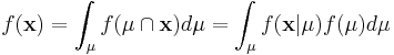
| - | Since <math>\mathbf{x}</math> is fixed, <math>f(\mathbf{x})</math> | + | Since <math>\mathbf{x}</math> is fixed, <math>f(\mathbf{x})</math> is a fixed number -- a "normalizing constant" so to ensure that the posterior density integrates to one. |
<math>f(\mathbf{x}) = \int_{\mu} f(\mu \cap \mathbf{x}) d\mu = \int_{\mu} f( \mathbf{x} | \mu ) f(\mu) d\mu </math> | <math>f(\mathbf{x}) = \int_{\mu} f(\mu \cap \mathbf{x}) d\mu = \int_{\mu} f( \mathbf{x} | \mu ) f(\mu) d\mu </math> | ||
Revision as of 20:13, 23 July 2009
Bayes Theorem
Bayes theorem, or "Bayes Rule" can be stated succinctly by the equality
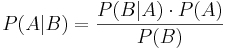
In words, "the probability of event A occurring given that event B occurred is equal to the probability of event B occurring given that event A occurred times the probability of event A occurring divided by the probability that event B occurs."
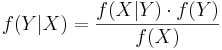
Bayes Theorem can also be written in terms of densities over continuous random variables. So, if  is some density, and X and Y are random variables, then we can say
What is commonly called Bayesian Statistics is a very special application of Bayes Theorem.
We will examine a number of examples in this Chapter, but to illustrate generally, imagine that x is a fixed collection of data that has been realized from under some known density, , that takes a parameter, μ, whose value is not certainly known.
Using Bayes Theorem we may write
In this formulation, we solve for  , the "posterior" density of the population parameter, μ.
For this we utilize the likelihood function of our data given our parameter,  , and, importantly, a density f(μ), that describes our "prior" belief in μ.
Since  is fixed,
  is a fixed number -- a "normalizing constant" so to ensure that the posterior density integrates to one.