AP Statistics Curriculum 2007 Contingency Fit
From Socr
(→ApoE and Alzheimer's disease (AD)) |
|||
| (31 intermediate revisions not shown) | |||
| Line 1: | Line 1: | ||
| - | ==[[AP_Statistics_Curriculum_2007 | General Advance-Placement (AP) Statistics Curriculum]] - Multinomial Experiments: Goodness-of-Fit == | + | ==[[AP_Statistics_Curriculum_2007 | General Advance-Placement (AP) Statistics Curriculum]] - Multinomial Experiments: Chi-Square Goodness-of-Fit == |
| - | + | Chi-Square Test is used to test if a data sample comes from a population with specific characteristics. The Chi-Square Goodness-of-Fit Test is applied to binned data (data put into classes or categories). In most situations, the data histogram or frequency histogram may be obtained and the Chi-Square Test may be applied to these (frequency) values. This test requires a sufficient sample size in order for the Chi-Square approximation to be valid. | |
| - | + | ||
| - | + | ||
| - | + | The [http://en.wikipedia.org/wiki/Kolmogorov-Smirnov_test Kolmogorov-Smirnov] is an alternative to the Chi-Square Goodness-of-Fit Test. The Chi-Square Goodness-of-Fit Test may also be applied to discrete distributions such as the Binomial and the Poisson. The Kolmogorov-Smirnov Test is restricted to continuous distributions. | |
| - | + | ||
| - | + | ==Motivational Example== | |
| + | [http://en.wikipedia.org/wiki/Mendelian_inheritance Mendel's Pea Experiment] relates to the transmission of hereditary characteristics from parent organisms to their offspring; it underlies much of genetics. Suppose a ''tall offspring'' is the event of interest and that the true proportion of tall peas (based on a 3:1 phenotypic ratio) is 3/4 or ''p = 0.75''. He would like to show that Mendel's data follow this 3:1 phenotypic ratio. | ||
| - | === | + | <center> |
| - | + | {| class="wikitable" style="text-align:center; width:25%" border="1" | |
| + | |- | ||
| + | | || '''Observed''' (O) || '''Expected''' (E) | ||
| + | |- | ||
| + | | '''Tall''' || 787 || 798 | ||
| + | |- | ||
| + | | '''Dwarf'''|| 277 || 266 | ||
| + | |} | ||
| + | </center> | ||
| - | + | ==Calculations== | |
| - | === | + | Suppose there were ''N = 1064'' data measurements with ''Observed(Tall) = 787'' and ''Observed(Dwarf) = 277''. These are the O’s (observed values). To calculate the E’s (expected values), we will take the hypothesized proportions under <math>H_o</math> and multiply them by the total sample size ''N''. Expected(Tall) = (0.75)(1064) = 798 and Expected(Dwarf) = (0.25)(1064) = 266. Quickly check to see if the expected total = N = 1064. |
| - | + | ||
| - | == | + | * The Hypotheses: |
| - | + | : <math>H_o</math>:P(tall) = 0.75 (No effect, follows a 3:1phenotypic ratio) | |
| + | :: P(dwarf) = 0.25 | ||
| + | : <math>H_a</math>: P(tall) ≠ 0.75 | ||
| + | ::P(dwarf) ≠ 0.25 | ||
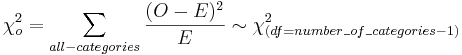
| - | * | + | * Test Statistics: |
| - | + | :<math>\chi_o^2 = \sum_{all-categories}{(O-E)^2 \over E} \sim \chi_{(df=number\_of\_categories - 1)}^2</math> | |
| - | = | + | |
| - | + | ||
| - | * | + | * P-values and Critical values for the [http://socr.stat.ucla.edu/htmls/SOCR_Distributions.html Chi-Square Distribution may be easily computed using SOCR Distributions]. |
| + | |||
| + | * Results: | ||
| + | For the Mendel's Pea Experiment, we can compute the Chi-Square Test Statistics to be: | ||
| + | : <math>\chi_o^2 = {(787-798)^2 \over 798} + {(277-266)^2 \over 266} = 0.152+0.455=0.607</math>. | ||
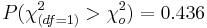
| + | : p-value=<math>P(\chi_{(df=1)}^2 > \chi_o^2)=0.436</math> | ||
| + | |||
| + | * [[SOCR_EduMaterials_AnalysisActivities_Chi_Goodness |SOCR Chi-Square Calculations]]: | ||
| + | |||
| + | <center>[[Image:SOCR_EBook_Dinov_ChiSquare_030108_Fig1.jpg|500px]]</center> | ||
| + | |||
| + | ==Assumptions== | ||
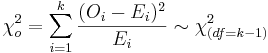
| + | The chi-square goodness-of-fit test requires that the data is divided into ''k'' bins and the test statistic is defined as | ||
| + | |||
| + | :<math>\chi_o^2 = \sum_{i=1}^k{(O_i-E_i)^2 \over E_i} \sim \chi_{(df=k - 1)}^2</math>, | ||
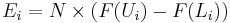
| + | where <math>O_i</math> is the observed frequency and <math>E_i</math> is the expected frequency for bin <math>1\leq i\leq k</math>. The expected counts may often be calculated by | ||
| + | |||
| + | : <math>E_i = N\times(F(U_i) - F(L_i))</math>, | ||
| + | where ''N'' is the total sample size, ''F'' is the cumulative distribution function (CDF) for the distribution being tested, <math>U_i</math> is the upper limit and <math>L_i</math> is the lower limit for class ''i''. | ||
| + | |||
| + | The chi-square test is sensitive to the choice of bins and the optimal choice for the bin-width may depend on the choice of the distribution. The chi-square test is valid if the data represent a random sample of at least 20 observations and the expected frequencies at each bin are at least 5. Otherwise, the distribution of the <math>\chi_o^2</math> statistics is not guaranteed to be <math>\chi_{k - 1}^2</math>, in general. In particular, the test may not be valid for small samples. If the expected counts are less than five for some bins, you may need to combine bins together to increase these counts. | ||
| + | |||
| + | ==Examples== | ||
| + | |||
| + | ===ApoE and Alzheimer's disease (AD)=== | ||
| + | |||
| + | ApoE (Apolipoprotein E) is a strong genetic risk factor for AD. About 40-65% of AD patients have at least one copy of the 4 allele, ApoE4, yet, at least 30% of patients with AD are ApoE4 negative and some ApoE4 homozygotes never develop the disease. People with two e4 alleles have up to 20 times the risk of developing AD. There is also evidence that the ApoE2 allele may serve a protective role in AD. Thus, the genotype most at risk for Alzheimer's disease and at an earlier age is the homozygous ApoE 4,4. The ApoE 3,4 genotype is at increased risk, genotype ApoE 3,3 is considered at normal risk for Alzheimer disease, and genotype ApoE 2,3 lowers the risk for Alzheimer disease. | ||
| + | |||
| + | Suppose we have a random sample of 100 AD patients and 100 asymptomatic age-matched controls. The table below illustrates the [http://en.wikipedia.org/wiki/Apolipoprotein_E#Alzheimer_disease expected distribution of the ApoE traits]. | ||
| + | |||
| + | <center> | ||
| + | {| class="wikitable" | ||
| + | |- | ||
| + | | colspan="6" align="center" | '''Estimated worldwide human allele frequencies of ApoE ''' | ||
| + | |- | ||
| + | | Allele || ε2 ||ε3 ||ε4||Total | ||
| + | |- | ||
| + | | General Frequency||8||78||14||100 | ||
| + | |- | ||
| + | | AD Frequency||4||59||37||100 | ||
| + | |- | ||
| + | | Total||12||137||51||200 | ||
| + | |} | ||
| + | </center> | ||
| + | |||
| + | Is there evidence of an association between genotype (alleles) and phenotype (disease)? What is the probability P(AD|ε2)? | ||
| + | |||
| + | ===Butterfly Hotspots=== | ||
| + | A hotspot is defined as a <math>10 km^2</math> area that is species rich (heavily populated by the species of interest). Suppose in a study of butterfly hotspots in a particular area of <math>10 km^2</math>, the number of butterfly hotspots in a sample of 2,588 is 165. In theory, 5% of the areas should be butterfly hotspots. Does the data provide evidence to suggest that the number of butterfly hotspots is increasing from the theoretical standards? Test using <math>\alpha= 0.01</math>. | ||
| + | |||
| + | ===Cell-Phone Usage=== | ||
| + | Of 250 randomly selected cell phone users, is there any evidence to show that there is a difference in area of home residence, defined as: Northern California (North); Southern California (South); or Out of State (Out)? Without further information suppose we have P(North) = 0.24, P(South) = 0.45, and P(Out) = 0.31. Is there any evidence suggesting different use of cell phones in these three groups of users? | ||
| + | |||
| + | ===Brain Cancer=== | ||
| + | Suppose 200 randomly selected cancer patients were asked if their primary diagnosis was brain cancer and if they owned a cell phone before their diagnosis. The results are presented in the table below: | ||
| + | |||
| + | <center> | ||
| + | {| class="wikitable" style="text-align:center; width:25%" border="1" | ||
| + | |- | ||
| + | | || || colspan=3| '''Brain cancer''' | ||
| + | |- | ||
| + | | || || '''Yes''' || '''No''' || '''Total''' | ||
| + | |- | ||
| + | | rowspan=3| '''Cell Phone Use''' || '''Yes''' || 18 || 80 || 98 | ||
| + | |- | ||
| + | | '''No''' || 7 || 95 || 102 | ||
| + | |- | ||
| + | | '''Total''' || 25 || 175 || 200 | ||
| + | |} | ||
| + | </center> | ||
| + | |||
| + | Does it seem like there is an association between brain cancer and cell phone use? | ||
| + | Of the brain cancer patients, 18 out of 25 (about 0.72) owned a cell phone before their diagnosis. | ||
| + | ''P(CP|BC) = 0.72'' is the estimated probability of patients owning a cell phone given that he or she has brain cancer. | ||
| + | |||
| + | Of the other cancer patients, 80 out of 175 (about 0.46) owned a cell phone before their diagnosis. | ||
| + | ''P(CP|NBC) = 0.46'' is the estimated probability of patients owning a cell phone given that he or she has a different type of cancer. | ||
| + | |||
| + | ===Chi-Square Die Experiment=== | ||
| + | The [[SOCR_EduMaterials_Activities_ChiSquareDiceExperiment | SOCR Chi-square die experiment]] illustrates the Chi-square goodness-of-fit test using two-dice. Suppose we are trying to prove that one of two dice is loaded. Let's call the first die the ''sampling-die'' and the second one the ''testing-die''. Using the [http://socr.ucla.edu/htmls/SOCR_Experiments.html Chi-Square dice applet] you can manually select the loading of the two dice (these can be the same or different loadings). The figure below illustrates this situation. Note that in this experiment, we've intentionally loaded the two dice in the opposite ways (look at the probability distributions in the testing and sampling tables in the image). Thus, we expect that the ''sampling-die'' will be a poor model for the (oppositely loaded) ''testing-die''. This is reflected in the results of the 10 experiments. All of them indicate statistically significant differences between the model (sampling-die) and the data (testing-die), which we can expect in this case. On the other hand, if we make the probability distributions of the two dice the same, a rejection of the null-hypothesis will only appear at the rate of the preset for α (0.02). | ||
| + | |||
| + | <center>[[Image:SOCR_EBook_Dinov_ChiSquare_042908_Fig2.jpg|500px]]</center> | ||
| + | |||
| + | ===Iris sepal and petal length=== | ||
| + | The [[SOCR_Data_052511_IrisSepalPetalClasses |Fisher's multivariate dataset on iris sepal and petal length]] provides another interesting example where we can look for how close are the petal or the sepal lengths of iris plant of different types. | ||
| + | |||
| + | ==Applications== | ||
| + | |||
| + | ===Polynomial Model Fitting=== | ||
| + | [http://socr.stat.ucla.edu/Applets.dir/SOCRCurveFitter.html This applet demonstrated the use of the Chi-Square test to assess quality of fitting a polynomial model (of any degree) to manually drawn curves]. | ||
<hr> | <hr> | ||
| - | === | + | ==[[EBook_Problems_Contingency_Fit|Problems]]== |
| - | * | + | |
| + | ==See also== | ||
| + | * [[SOCR_EduMaterials_Activities_BMI_Modeling_Activity|SOCR BMI Modeling Activity]] | ||
| + | * [[SOCR_EduMaterials_AnalysisActivities_Chi_Goodness| SOCR Chi-Square Goodness-of-Fit Test]] | ||
<hr> | <hr> | ||
Current revision as of 19:01, 4 April 2013
Contents |
General Advance-Placement (AP) Statistics Curriculum - Multinomial Experiments: Chi-Square Goodness-of-Fit
Chi-Square Test is used to test if a data sample comes from a population with specific characteristics. The Chi-Square Goodness-of-Fit Test is applied to binned data (data put into classes or categories). In most situations, the data histogram or frequency histogram may be obtained and the Chi-Square Test may be applied to these (frequency) values. This test requires a sufficient sample size in order for the Chi-Square approximation to be valid.
The Kolmogorov-Smirnov is an alternative to the Chi-Square Goodness-of-Fit Test. The Chi-Square Goodness-of-Fit Test may also be applied to discrete distributions such as the Binomial and the Poisson. The Kolmogorov-Smirnov Test is restricted to continuous distributions.
Motivational Example
Mendel's Pea Experiment relates to the transmission of hereditary characteristics from parent organisms to their offspring; it underlies much of genetics. Suppose a tall offspring is the event of interest and that the true proportion of tall peas (based on a 3:1 phenotypic ratio) is 3/4 or p = 0.75. He would like to show that Mendel's data follow this 3:1 phenotypic ratio.
| Observed (O) | Expected (E) | |
| Tall | 787 | 798 |
| Dwarf | 277 | 266 |
Calculations
Suppose there were N = 1064 data measurements with Observed(Tall) = 787 and Observed(Dwarf) = 277. These are the O’s (observed values). To calculate the E’s (expected values), we will take the hypothesized proportions under Ho and multiply them by the total sample size N. Expected(Tall) = (0.75)(1064) = 798 and Expected(Dwarf) = (0.25)(1064) = 266. Quickly check to see if the expected total = N = 1064.
- The Hypotheses:
- Ho:P(tall) = 0.75 (No effect, follows a 3:1phenotypic ratio)
- P(dwarf) = 0.25
- Ha: P(tall) ≠ 0.75
- P(dwarf) ≠ 0.25
- Test Statistics:
- P-values and Critical values for the Chi-Square Distribution may be easily computed using SOCR Distributions.
- Results:
For the Mendel's Pea Experiment, we can compute the Chi-Square Test Statistics to be:
-
 .
.
- p-value=

Assumptions
The chi-square goodness-of-fit test requires that the data is divided into k bins and the test statistic is defined as
 ,
,
where Oi is the observed frequency and Ei is the expected frequency for bin  . The expected counts may often be calculated by
-
 ,
,
where N is the total sample size, F is the cumulative distribution function (CDF) for the distribution being tested, Ui is the upper limit and Li is the lower limit for class i.
The chi-square test is sensitive to the choice of bins and the optimal choice for the bin-width may depend on the choice of the distribution. The chi-square test is valid if the data represent a random sample of at least 20 observations and the expected frequencies at each bin are at least 5. Otherwise, the distribution of the  statistics is not guaranteed to be
  , in general. In particular, the test may not be valid for small samples. If the expected counts are less than five for some bins, you may need to combine bins together to increase these counts.
Examples
ApoE and Alzheimer's disease (AD)
ApoE (Apolipoprotein E) is a strong genetic risk factor for AD. About 40-65% of AD patients have at least one copy of the 4 allele, ApoE4, yet, at least 30% of patients with AD are ApoE4 negative and some ApoE4 homozygotes never develop the disease. People with two e4 alleles have up to 20 times the risk of developing AD. There is also evidence that the ApoE2 allele may serve a protective role in AD. Thus, the genotype most at risk for Alzheimer's disease and at an earlier age is the homozygous ApoE 4,4. The ApoE 3,4 genotype is at increased risk, genotype ApoE 3,3 is considered at normal risk for Alzheimer disease, and genotype ApoE 2,3 lowers the risk for Alzheimer disease.
Suppose we have a random sample of 100 AD patients and 100 asymptomatic age-matched controls. The table below illustrates the expected distribution of the ApoE traits.
| Estimated worldwide human allele frequencies of ApoE | |||||
| Allele | ε2 | ε3 | ε4 | Total | |
| General Frequency | 8 | 78 | 14 | 100 | |
| AD Frequency | 4 | 59 | 37 | 100 | |
| Total | 12 | 137 | 51 | 200 | |
Is there evidence of an association between genotype (alleles) and phenotype (disease)? What is the probability P(AD|ε2)?
Butterfly Hotspots
A hotspot is defined as a 10km2 area that is species rich (heavily populated by the species of interest). Suppose in a study of butterfly hotspots in a particular area of 10km2, the number of butterfly hotspots in a sample of 2,588 is 165. In theory, 5% of the areas should be butterfly hotspots. Does the data provide evidence to suggest that the number of butterfly hotspots is increasing from the theoretical standards? Test using α = 0.01.
Cell-Phone Usage
Of 250 randomly selected cell phone users, is there any evidence to show that there is a difference in area of home residence, defined as: Northern California (North); Southern California (South); or Out of State (Out)? Without further information suppose we have P(North) = 0.24, P(South) = 0.45, and P(Out) = 0.31. Is there any evidence suggesting different use of cell phones in these three groups of users?
Brain Cancer
Suppose 200 randomly selected cancer patients were asked if their primary diagnosis was brain cancer and if they owned a cell phone before their diagnosis. The results are presented in the table below:
| Brain cancer | ||||
| Yes | No | Total | ||
| Cell Phone Use | Yes | 18 | 80 | 98 |
| No | 7 | 95 | 102 | |
| Total | 25 | 175 | 200 | |
Does it seem like there is an association between brain cancer and cell phone use? Of the brain cancer patients, 18 out of 25 (about 0.72) owned a cell phone before their diagnosis. P(CP|BC) = 0.72 is the estimated probability of patients owning a cell phone given that he or she has brain cancer.
Of the other cancer patients, 80 out of 175 (about 0.46) owned a cell phone before their diagnosis. P(CP|NBC) = 0.46 is the estimated probability of patients owning a cell phone given that he or she has a different type of cancer.
Chi-Square Die Experiment
The SOCR Chi-square die experiment illustrates the Chi-square goodness-of-fit test using two-dice. Suppose we are trying to prove that one of two dice is loaded. Let's call the first die the sampling-die and the second one the testing-die. Using the Chi-Square dice applet you can manually select the loading of the two dice (these can be the same or different loadings). The figure below illustrates this situation. Note that in this experiment, we've intentionally loaded the two dice in the opposite ways (look at the probability distributions in the testing and sampling tables in the image). Thus, we expect that the sampling-die will be a poor model for the (oppositely loaded) testing-die. This is reflected in the results of the 10 experiments. All of them indicate statistically significant differences between the model (sampling-die) and the data (testing-die), which we can expect in this case. On the other hand, if we make the probability distributions of the two dice the same, a rejection of the null-hypothesis will only appear at the rate of the preset for α (0.02).

Iris sepal and petal length
The Fisher's multivariate dataset on iris sepal and petal length provides another interesting example where we can look for how close are the petal or the sepal lengths of iris plant of different types.
Applications
Polynomial Model Fitting
Problems
See also
- SOCR Home page: http://www.socr.ucla.edu
Translate this page:
