AP Statistics Curriculum 2007 EDA Center
From Socr
m (→Other Measures of Centrality) |
|||
| Line 50: | Line 50: | ||
* '''K-times trimmed mean''': <math>\bar{y}_{t,k}={1\over n-2k}\sum_{i=k+1}^{n-k}{y_{(i)}}</math>, where <math>k\geq 0</math> is the trim-factor (large k, yield less varient estimates of center), and <math>y_{(i)}</math> are the order statistics (small to large). That is, we remove the smallest and the largest ''k'' observations from the sample, before we compute the arithmetic average. | * '''K-times trimmed mean''': <math>\bar{y}_{t,k}={1\over n-2k}\sum_{i=k+1}^{n-k}{y_{(i)}}</math>, where <math>k\geq 0</math> is the trim-factor (large k, yield less varient estimates of center), and <math>y_{(i)}</math> are the order statistics (small to large). That is, we remove the smallest and the largest ''k'' observations from the sample, before we compute the arithmetic average. | ||
| - | * '''Windsorized k-times mean''': The Windsorirized k-times mean is defined similarly by <math>\bar{y}_{t,k}={1\over n}( k\times y_{(k)}+\sum_{i=k+1}^{n-k-1}{y_{(i)}}+k\times y_{(n-k)}</math>, where <math>k\geq 0</math> is the trim-factor and <math>y_{(i)}</math> are the order statistics (small to large). In this case, before we compute the arithmetic average, we replace the ''k'' smallest and the ''k'' largest observations with the k<sup>th</sup> and (n-k)<sup>th</sup> largest obsarvations, respectively. | + | * '''Windsorized k-times mean''': The Windsorirized k-times mean is defined similarly by <math>\bar{y}_{t,k}={1\over n}( k\times y_{(k)}+\sum_{i=k+1}^{n-k-1}{y_{(i)}}+k\times y_{(n-k)})</math>, where <math>k\geq 0</math> is the trim-factor and <math>y_{(i)}</math> are the order statistics (small to large). In this case, before we compute the arithmetic average, we replace the ''k'' smallest and the ''k'' largest observations with the k<sup>th</sup> and (n-k)<sup>th</sup> largest obsarvations, respectively. |
<hr> | <hr> | ||
| + | |||
===References=== | ===References=== | ||
* [http://www.stat.ucla.edu/%7Edinov/courses_students.dir/07/Fall/STAT13.1.dir/STAT13_notes.dir/lecture02.pdf Lecture notes on EDA] | * [http://www.stat.ucla.edu/%7Edinov/courses_students.dir/07/Fall/STAT13.1.dir/STAT13_notes.dir/lecture02.pdf Lecture notes on EDA] | ||
Revision as of 21:52, 6 March 2008
Contents |
General Advance-Placement (AP) Statistics Curriculum - Central Tendency
Measurements of Central Tendency
There are three main features of all populations (or data samples) that are always critical in understanding and interpreting their distributions. These characteristics are Center, Spread and Shape. The main measure of centrality are mean, median and mode.
Suppose we are interested in the long-jump performance of some students. We can carry an experiment by randomly selecting 8 male statistics students and ask them to perform the standing long jump. In reality every student participated, but for the ease of calculations below we will focus on these eight students. The long jumps were as follows:
| 74 | 78 | 106 | 80 | 68 | 64 | 60 | 76 |
Mean
The sample-mean is the arithmetic average of a finite sample of numbers. In the long-jump example. The sample-mean is calculated as follows:

Median
The sample-median can be thought of as the point that divides a distribution in half (50/50). The following steps are used to find the sample-median:
- Arrange the data in ascending order
- If the sample size is odd, the median is the middle value of the ordered collection
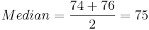
- If the sample size is even, the median is the average of the middle two values in the ordered collection.
For the long-jump data above we have:
- Ordered data:
| 60 | 64 | 68 | 74 | 76 | 78 | 80 | 106 |
-
 .
.
Mode(s)
The modes represent the most frequently occurring values (The numbers that appear the most). The term mode is applied both to probability distributions and to collections of experimental data.
For instance, for the Hot dogs data file, there appear to be 3 modes for the calorie variable! This is evident by the histogram of the Calorie content of all hotdogs, shown in the image below. Note the clear separation of the calories into 3 distinct sub-populations - the highest points in these three sub-populations are the three modes for these data.

Resistance
A statistic is said to be resistant if the value of the statistic is relatively unchanged by changes in a small portion of the data. Referencing the formulas for the median, mean and mode which statistic seems to be more resistant?
If you remove the student with the long jump distance of 106 and recalculate the median and mean, which one is altered less (therefore is more resistant)? Notice that the mean is very sensitive to outliers and atypical observations, and hence less resistant than the median.
Other Measures of Centrality
The following two sample meausres of population centrality estimate resemble the calculations of the mean, however they are much more resistant to change in the presence of outliers.
- K-times trimmed mean:
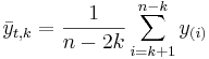 , where
  is the trim-factor (large k, yield less varient estimates of center), and y(i) are the order statistics (small to large). That is, we remove the smallest and the largest k observations from the sample, before we compute the arithmetic average.
- Windsorized k-times mean: The Windsorirized k-times mean is defined similarly by
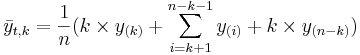 , where is the trim-factor and y(i) are the order statistics (small to large). In this case, before we compute the arithmetic average, we replace the k smallest and the k largest observations with the kth and (n-k)th largest obsarvations, respectively.
References
- SOCR Home page: http://www.socr.ucla.edu
Translate this page:
