AP Statistics Curriculum 2007 Fisher F
From Socr
Contents |
General Advance-Placement (AP) Statistics Curriculum - Fisher's F Distribution
Fisher's F Distribution
Commonly used as the null distribution of a test statistic, such as in analysis of variance ANOVA. Relationship to the t-distribution and beta Distribution.
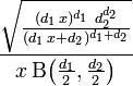
PDF:
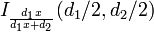
CDF:
Mean:
 for d2 > 2
Median:
None
Mode:
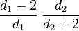 for d1 > 2
Variance:
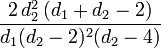 for d2 > 4
Support:
Moment Generating Function
Does Not Exist
Applications
Example
We want to examine the effect of three different brands of gasoline on gas mileage using an alpha value of 0.05. We will have 6 observations for each of the 3 gasoline brands. Gas mileage figures are as follows:
| Brand A | Brand B | Brand C |
|---|---|---|
| 29 | 30 | 28 |
| 30 | 31 | 29 |
| 29 | 32 | 28 |
| 28 | 29 | 26 |
| 30 | 31 | 30 |
| 28 | 33 | 29 |
Our null hypothesis, H0, is that the three brands of gasoline will yield the same amount of gas mileage, on average.
First, we find the F-ratio:
Step 1: Calculate the mean for each brand:
Brand A: 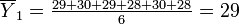
Brand B: 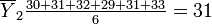
Brand C: 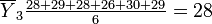
Step 2: Calculate the overall mean:

Step 3: Calculate the Between-Group Sum of Squares:

Where n is the number of observations per group.
The between-group degrees of freedom is one less than the number of groups: 3-1=2.
Therefore, the between-group mean square value, MSB, is 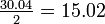
Step 4: Calculate the Within-Group Sum of Squares:
We start by subtracting each observation by its group mean:
| Brand A | Brand B | Brand C |
|---|---|---|
| 29-29=0 | 30-31=-1 | 28-28=0 |
| 30-29=1 | 31-31=0 | 29-28=1 |
| 29-29=0 | 32-31=1 | 28-28=0 |
| 28-29=-1 | 29-31=-2 | 26-28=-2 |
| 30-29=1 | 31-31=0 | 30-28=2 |
| 28-29=-1 | 33-31=2 | 29-28=1 |
The Within-Group Sum of Squares, SSw, is the sum of the squares of the values in the previous table:
0 + 1 + 0 + 1 + 0 + 1 + 0 + 1 + 0 + 1 + 4 + 4 + 1 + 0 + 4 + 1 + 4 + 1 = 24
The Within-Group degrees of freedom is the number of groups times 1 less the number of observations per group:
3(6 − 1) = 15
The Within-Group Mean Square Value, MSW is: 
Step 5: Finally, the F-Ratio is:
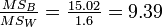
The F critical value is the value that the test statistic must exceed in order to reject the H0. In this case, Fcrit(2,15) = 3.68 at α = 0.05. Since F=9.39>3.68, we reject H0 at the 5% significance level, concluding that there is a difference in gas mileage between the gasoline brands.
We can find the critical F-value using the SOCR F Distribution Calculator:

SOCR Links
http://www.distributome.org/ -> SOCR -> Distributions -> Fisher’s F
http://www.distributome.org/ -> SOCR -> Distributions -> Fisher’s F Distribution
http://www.distributome.org/ -> SOCR -> Functors -> Fisher’s F Distribution
http://www.distributome.org/ -> SOCR -> Analyses -> ANOVA – One Way
http://www.distributome.org/ -> SOCR -> Analyses -> ANOVA – Two Way
SOCR F-Distribution Calculator (http://socr.ucla.edu/htmls/dist/Fisher_Distribution.html)
- SOCR Home page: http://www.socr.ucla.edu
Translate this page:
