AP Statistics Curriculum 2007 GLM Regress
From Socr
(→Regression Coefficients Inference) |
|||
| (14 intermediate revisions not shown) | |||
| Line 1: | Line 1: | ||
==[[AP_Statistics_Curriculum_2007 | General Advance-Placement (AP) Statistics Curriculum]] - Regression == | ==[[AP_Statistics_Curriculum_2007 | General Advance-Placement (AP) Statistics Curriculum]] - Regression == | ||
| - | As we discussed in the [[AP_Statistics_Curriculum_2007_GLM_Corr |Correlation section]], many applications involve the analysis of relationships between two, or more, variables involved in the process of interest. Suppose we have bivariate data (''X'' and ''Y'') of a process and we are interested | + | As we discussed in the [[AP_Statistics_Curriculum_2007_GLM_Corr |Correlation section]], many applications involve the analysis of relationships between two, or more, variables involved in the process of interest. Suppose we have bivariate data (''X'' and ''Y'') of a process and we are interested in determining the linear relation between X and Y (e.g., determining a straight line that best fits the pairs of data (''X,Y'')). A linear relationship between ''X'' and ''Y'' will give us the power to make predictions - i.e., given a value of ''X'' predict a corresponding ''Y'' response. Note that in this design, data consists of paired observations (''X,Y'') - for example, the [[SOCR_Data_Dinov_021708_Earthquakes | Longitude and Latitude of the SOCR Earthquake dataset]]. |
===Lines in 2D=== | ===Lines in 2D=== | ||
| Line 20: | Line 20: | ||
* Y is an observed variable and X is specified by the researcher - e.g., Y is hair growth after X months, for individuals at certain dose levels of hair growth cream. | * Y is an observed variable and X is specified by the researcher - e.g., Y is hair growth after X months, for individuals at certain dose levels of hair growth cream. | ||
| - | * X and Y are both observed variables - e.g., [[SOCR_Data_Dinov_020108_HeightsWeights | | + | * X and Y are both observed variables - e.g., [[SOCR_Data_Dinov_020108_HeightsWeights | height (Y) and weight (X)]] for 20 randomly selected individuals from the population. |
Suppose we have ''n'' pairs ''(X,Y)'', {<math>X_1, X_2, X_3, \cdots, X_n</math>} and {<math>Y_1, Y_2, Y_3, \cdots, Y_n</math>}, of observations of the same process. If a [[SOCR_EduMaterials_Activities_ScatterChart |scatterplot]] of the data suggests a general linear trend, it would be reasonable to fit a line to the data. The main question is how to determine the best line? | Suppose we have ''n'' pairs ''(X,Y)'', {<math>X_1, X_2, X_3, \cdots, X_n</math>} and {<math>Y_1, Y_2, Y_3, \cdots, Y_n</math>}, of observations of the same process. If a [[SOCR_EduMaterials_Activities_ScatterChart |scatterplot]] of the data suggests a general linear trend, it would be reasonable to fit a line to the data. The main question is how to determine the best line? | ||
====[[AP_Statistics_Curriculum_2007_GLM_Corr#Airfare_Example |Airfare Example]]==== | ====[[AP_Statistics_Curriculum_2007_GLM_Corr#Airfare_Example |Airfare Example]]==== | ||
| - | We can see from the [[SOCR_EduMaterials_Activities_ScatterChart |scatterplot]] that greater distance is associated with higher airfare. In other words airports that tend to be further from Baltimore tend to | + | We can see from the [[SOCR_EduMaterials_Activities_ScatterChart |scatterplot]] that [[AP_Statistics_Curriculum_2007_GLM_Corr#Airfare_Example | greater distance is associated with higher airfare]]. In other words airports that tend to be further from Baltimore tend to have more expensive airfare. To decide on the best fitting line, we use the '''least-squares method''' to fit the least squares (regression) line. |
<center>[[Image:SOCR_EBook_Dinov_GLM_Regr_021708_Fig1.jpg|500px]]</center> | <center>[[Image:SOCR_EBook_Dinov_GLM_Regr_021708_Fig1.jpg|500px]]</center> | ||
====Estimating the Best Linear Fit==== | ====Estimating the Best Linear Fit==== | ||
| - | The parameters of the linear regression line, <math>Y = a + bX</math>, can be estimated using [http://en.wikipedia.org/wiki/Ordinary_Least_Squares Least Squares]. | + | The parameters of the linear regression line, <math>Y = a + bX</math>, can be estimated using [http://en.wikipedia.org/wiki/Ordinary_Least_Squares Least Squares]. The least squares technique finds the line that minimizes the sum of the squares of the regression '''residuals''', <math>\hat{\varepsilon_i}=\hat{y}_{i}-y_i</math>, <math> \sum_{i=1}^N {\hat{\varepsilon_i}^2} = \sum_{i=1}^N (\hat{y}_{i}-y_i)^2 </math>, where <math>y_i</math> and <math>\hat{y}_{i}=a+bx_i</math> are the observed and the predicted values of ''Y'' for <math>x_i</math>. |
The minimization problem can be solved using calculus, by finding the first order partial derivatives and setting them equal to zero. The solution gives the slope and y-intercept of the regressions line: | The minimization problem can be solved using calculus, by finding the first order partial derivatives and setting them equal to zero. The solution gives the slope and y-intercept of the regressions line: | ||
| Line 50: | Line 50: | ||
If the error terms are Normally distributed, the estimate of the slope coefficient has a normal distribution with mean equal to '''b''' and ''standard error'' given by: | If the error terms are Normally distributed, the estimate of the slope coefficient has a normal distribution with mean equal to '''b''' and ''standard error'' given by: | ||
| - | : <math> s_ \hat{b} = \sqrt { {1\over (N-2)} \frac {\sum_{i=1}^N \hat{\varepsilon_i}^2} {\sum_{i=1}^N (x_i - \bar{x})^2} }</math>. | + | :: <math> SE(\hat{b}) = s_ \hat{b} = \sqrt { {1\over (N-2)} \frac {\sum_{i=1}^N \hat{\varepsilon_i}^2} {\sum_{i=1}^N (x_i - \bar{x})^2} }</math>. |
| - | A confidence interval for ''b'' can be created using a [[AP_Statistics_Curriculum_2007_StudentsT | T-distribution with N-2 degrees of freedom]]: | + | * A confidence interval for ''b'' can be created using a [[AP_Statistics_Curriculum_2007_StudentsT | T-distribution with N-2 degrees of freedom]]: |
| - | :<math> [ \hat{b} - s_ \hat{b} t_{N-2} | + | ::<math> [ \hat{b} - s_ \hat{b} t_{(\alpha/2, N-2)},\hat{b} + s_ \hat{b} t_{(\alpha/2, N-2)}] </math> |
| + | |||
| + | * The corresponding test for the regression slope coefficient ''b'' is analogously computed (<math>H_o: b=b_o</math> vs. <math>H_a: b \not= b_0</math>, frequently <math>b_0 = 0</math>) | ||
| + | |||
| + | ::<math> t_o = {\hat{b} - b_o \over s_ \hat{b} } \sim T_{df=N-2}. </math> | ||
===Hands-on Example=== | ===Hands-on Example=== | ||
| Line 68: | Line 72: | ||
===Earthquake Example=== | ===Earthquake Example=== | ||
| - | Use the [[SOCR_Data_Dinov_021708_Earthquakes | SOCR Earthquake Dataset]] to determine the best- | + | Use the [[SOCR_Data_Dinov_021708_Earthquakes | SOCR Earthquake Dataset]] to determine the best-linear fit between the [http://nationalatlas.gov/articles/mapping/a_latlong.html Longitude] and the [http://nationalatlas.gov/articles/mapping/a_latlong.html Latitude] of the California Earthquakes since 1900. What is the interpretation of this regression line ([http://en.wikipedia.org/wiki/San_Andreas_Fault San Andreas fault]?). You can see the [http://socr.ucla.edu/docs/resources/SOCR_Data/SOCR_Earthquake5Data_GoogleMap.html SOCR Geomap of these Earthquakes]. The image below shows how to use the [[SOCR_EduMaterials_AnalysisActivities_SLR |Simple Linear regression]] in [http://socr.ucla.edu/htmls/SOCR_Analyses.html SOCR Analyses] to calculate the regression line: |
| + | : <math>Latitude = -40.149 -0.6457\times Longitude</math> | ||
<center>[[Image:SOCR_EBook_Dinov_GLM_Regr_021708_Fig2.jpg|500px]]</center> | <center>[[Image:SOCR_EBook_Dinov_GLM_Regr_021708_Fig2.jpg|500px]]</center> | ||
| + | |||
| + | ===Hands-on Example=== | ||
| + | Compute by hand the regression line between X and Y and validate your results using [http://socr.ucla.edu/htmls/SOCR_Analyses.html the SOCR Regression Analysis]. | ||
| + | <center> | ||
| + | {| class="wikitable" style="text-align:center; width:75%" border="1" | ||
| + | |- | ||
| + | | X || Y in cm || <math>x_i-\bar{x}</math> || <math>y_i-\bar{y}</math> || <math>(x_i-\bar{x})^2</math> || <math>(y_i-\bar{y})^2</math> || <math>(x_i-\bar{x})(y_i-\bar{y})</math> | ||
| + | |- | ||
| + | | -1 || 0 || -3 || -0.5 || 9 || 0.25 || 1.5 | ||
| + | |- | ||
| + | | 2 || -1 || 0 || -1.5 || 0 || 2.25 || 0 | ||
| + | |- | ||
| + | | 3 || 1 || 1 || 0.5 || 1 || 0.25 || 0.5 | ||
| + | |- | ||
| + | | 4 || 2 || 2 || 1.5 || 4 || 2.25 || 3 | ||
| + | |- | ||
| + | | <math>\bar{x}</math> || <math>\bar{y}</math> || || || || || | ||
| + | |} | ||
| + | </center> | ||
<hr> | <hr> | ||
| - | === | + | |
| + | ===[[EBook_Problems_GLM_Regress|Problems]]=== | ||
| + | |||
| + | ===See also=== | ||
| + | * [[SOCR_EduMaterials_AnalysisActivities_SLR| SOCR Linear Regression Activity]] | ||
<hr> | <hr> | ||
Current revision as of 19:19, 13 August 2012
Contents |
General Advance-Placement (AP) Statistics Curriculum - Regression
As we discussed in the Correlation section, many applications involve the analysis of relationships between two, or more, variables involved in the process of interest. Suppose we have bivariate data (X and Y) of a process and we are interested in determining the linear relation between X and Y (e.g., determining a straight line that best fits the pairs of data (X,Y)). A linear relationship between X and Y will give us the power to make predictions - i.e., given a value of X predict a corresponding Y response. Note that in this design, data consists of paired observations (X,Y) - for example, the Longitude and Latitude of the SOCR Earthquake dataset.
Lines in 2D
There are 3 types of lines in 2D planes - Vertical Lines, Horizontal Lines and Oblique Lines. In general, the mathematical representation of lines in 2D is given by equations like aX + bY = c, most frequently expressed as Y = aX + b, provides the line is not vertical.
Recall that there is a one-to-one correspondence between any line in 2D and (linear) equations of the form
- If the line is vertical (X1 = X2): X = X1;
- If the line is horizontal (Y1 = Y2): Y = Y1;
- Otherwise (oblique line):
 , (for
  and
and  )
)
where (X1,Y1) and (X2,Y2) are two points on the line of interest (2-distinct points in 2D determine a unique line).
- Try drawing the following lines manually and using this applet:
- Y=2X+1
- Y=-3X-5
Linear Modeling - Regression
There are two contexts for regression:
- Y is an observed variable and X is specified by the researcher - e.g., Y is hair growth after X months, for individuals at certain dose levels of hair growth cream.
- X and Y are both observed variables - e.g., height (Y) and weight (X) for 20 randomly selected individuals from the population.
Suppose we have n pairs (X,Y), { } and {
 }, of observations of the same process. If a scatterplot of the data suggests a general linear trend, it would be reasonable to fit a line to the data. The main question is how to determine the best line?
Airfare Example
We can see from the scatterplot that greater distance is associated with higher airfare. In other words airports that tend to be further from Baltimore tend to have more expensive airfare. To decide on the best fitting line, we use the least-squares method to fit the least squares (regression) line.

Estimating the Best Linear Fit
The parameters of the linear regression line, Y = a + bX, can be estimated using Least Squares. The least squares technique finds the line that minimizes the sum of the squares of the regression residuals,  ,
, 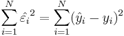 , where yi and
  are the observed and the predicted values of Y for xi.
The minimization problem can be solved using calculus, by finding the first order partial derivatives and setting them equal to zero. The solution gives the slope and y-intercept of the regressions line:
- Regression line Slope:
-
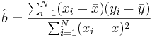
-
 , where ρX,Y is the correlation coefficient.
- Y-intercept:

- Properties of the least square line:
- The line goes through the point

- The sum of the residuals is equal to zero
- The estimates are unbiased (their expected values are equal to the real slope and intercept values).
- The line goes through the point
Regression Coefficients Inference
If the error terms are Normally distributed, the estimate of the slope coefficient has a normal distribution with mean equal to b and standard error given by:
-
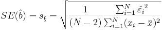 .
.
-
- A confidence interval for b can be created using a T-distribution with N-2 degrees of freedom:
![[ \hat{b} - s_ \hat{b} t_{(\alpha/2, N-2)},\hat{b} + s_ \hat{b} t_{(\alpha/2, N-2)}]](/socr/uploads/math/9/7/f/97fb851896b79e5d8eb45162cd0c6390.png)
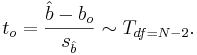
- The corresponding test for the regression slope coefficient b is analogously computed (Ho:b = bo vs.
 , frequently b0 = 0)
Hands-on Example
Suppose we have 3 sample of points {(1,-1),(2,4),(6,3)}. The mean of X is 3 and the mean of Y is 2. The slope coefficient estimate is given by:

The standard error of the slope coefficient (b) is 0.866. A 95% confidence interval is given by:
- CI(b): [0.5 - 0.866 x 12.7062, 0.5 + 0.866 x 12.7062] = [-10.504, 11.504].
Earthquake Example
Use the SOCR Earthquake Dataset to determine the best-linear fit between the Longitude and the Latitude of the California Earthquakes since 1900. What is the interpretation of this regression line (San Andreas fault?). You can see the SOCR Geomap of these Earthquakes. The image below shows how to use the Simple Linear regression in SOCR Analyses to calculate the regression line:


Hands-on Example
Compute by hand the regression line between X and Y and validate your results using the SOCR Regression Analysis.
| X | Y in cm |  |  |  |  | 
|
| -1 | 0 | -3 | -0.5 | 9 | 0.25 | 1.5 |
| 2 | -1 | 0 | -1.5 | 0 | 2.25 | 0 |
| 3 | 1 | 1 | 0.5 | 1 | 0.25 | 0.5 |
| 4 | 2 | 2 | 1.5 | 4 | 2.25 | 3 |
 |  |
Problems
See also
- SOCR Home page: http://www.socr.ucla.edu
Translate this page:
