AP Statistics Curriculum 2007 Infer 2Means Indep
From Socr
Contents
|
General Advance-Placement (AP) Statistics Curriculum - Inferences about Two Means: Independent Samples
In the previous section we discussed the inference on two paired random samples. Now, we show how to do inference on two independent samples.
Independent Samples Designs
Independent samples designs refer to design of experiments or observations where all measurements are individually independent from each other within their groups and the groups are independent. The groups may be drawn from different populations with different distribution characteristics.
Background
- Recall that for a random sample {
 } of the process, the population mean may be estimated by the sample average,
  .
.
- The standard error of
 is given by
  .
.
Analysis Protocol for Independent Designs
To study independent samples, we would like to examine the differences between two group means. Suppose { } and {
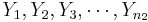 } represent the two independent samples. Then we want to study the differences of the two group means relative to the internal sample variations. If the two samples were drawn from populations that had different centers, then we would expect that the two sample averages will be distinct.
Large Samples
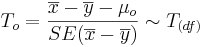
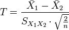
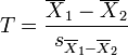
- Significance Testing: We have a standard null-hypothesis Ho:μX − μY = μo (e.g., μo = 0). Then the test statistics is:
-
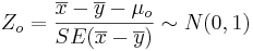 .
.
-
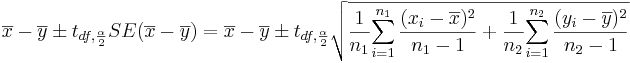
- Confidence Intervals: (1 − α)100% confidence interval for μ1 − μ2 will be
-
 . Note that the
 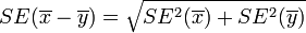 , as the samples are independent. Also,
  is the critical value for a Standard Normal distribution at
  .
.
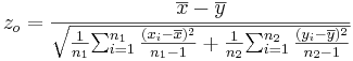
Small Samples
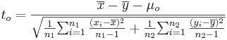
- Significance Testing: Again, we have a standard null-hypothesis Ho:μX − μY = μo (e.g., μo = 0). Then the test statistics is:
-
 .
.
- The degrees of freedom (df) is:
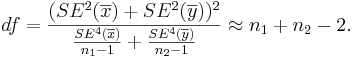 Always round down the degrees of freedom to the next smaller integer.
-
- Confidence Intervals: (1 − α)100% confidence interval for μ1 − μ2 will be
-
 . Note that the , as the samples are independent.
- The degrees of freedom is: Always round down the degrees of freedom to the next smaller integer. Also,
 is the critical value for a Student's T distribution at .
Example
Nine observations of surface soil pH were made at two different locations. Does the data suggest that the true mean soil pH values differs for the two locations? Formulate testable hypothesis and make inference about the effect of the treatment at α = 0.05. Check any necessary assumptions for the validity of your test.
Data in row format
| Location 1 | 8.1,7.89,8,7.85,8.01,7.82,7.99,7.8,7.93 |
| Location 2 | 7.85,7.3,7.73,7.27,7.58,7.27,7.5,7.23,7.41 |
Data in column format
| Index | Location 1 | Location 2 |
|---|---|---|
| 1 | 8.10 | 7.85 |
| 2 | 7.89 | 7.30 |
| 3 | 8.00 | 7.73 |
| 4 | 7.85 | 7.27 |
| 5 | 8.01 | 7.58 |
| 6 | 7.82 | 7.27 |
| 7 | 7.99 | 7.50 |
| 8 | 7.80 | 7.23 |
| 9 | 7.93 | 7.41 |
| Mean | 7.9322 | 7.4600 |
| SD | 0.1005 | 0.2220 |
Exploratory Data Analysis
We begin first by exploring the data visually using various SOCR EDA Tools.
- Line Chart of the two samples

- Box-And-Whisker Plot of the two samples

Inference
- Null Hypothesis: Ho:μ1 − μ2 = 0
- (Two-sided) alternative Research Hypotheses:
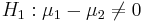 .
.
- Test statistics: We can use the sample summary statistics to compute the degrees of freedom and the T-statistic
- The degrees of freedom is:
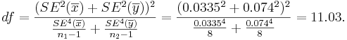 So, we round down df=11.
-
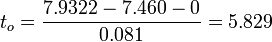 .
.
- p − value = P(T(df = 11) > To = 5.829) = 0.00003 for this (two-sided) test. Therefore, we can reject the null hypothesis at α = 0.05! The left white area at the tails of the T(df=11) distribution depicts graphically the probability of interest, which represents the strength of the evidence (in the data) against the Null hypothesis. In this case, this area is 0.00003, which is much smaller than the initially set Type I error α = 0.05 and we reject the null hypothesis.

- You can also use the SOCR Analyses (Two-Independent Samples T-Test) to carry out these calculations as shown in the figure below.

- This SOCR Two-Sample Independent T-test Activity provides additional hands-on demonstrations of the two-sample hypothesis testing.
- 95% = (1 − 0.05)100% (α = 0.05) Confidence interval:
- CI(μ1 − μ2):
![CI: {7.932-7.460 \pm 2.201\times 0.081 }= [0.294 ; 0.650].](/socr/uploads/math/2/8/6/286be017d1a16fb1a788ec44a8c2b566.png)
Conclusion
These data show that there is a statistically significant mean difference in the pH of Location 1 and Location 2 (p < 0.001).
Independent T-test Validity
Both the confidence intervals and the hypothesis testing methods in the independent-sample design require Normality of both samples. If the sample sizes are large (say >50), Normality is not as critical, as the CLT implies the sampling distributions of the means are approximately Normal. If these parametric assumptions are invalid we must use a non-parametric (distribution free test), even if the latter is less powerful.
The plots below indicate that Normal assumptions are not unreasonable for these data, and hence we may be justified in using the two independent sample T-tests in this case.
- QQ-Normal plot of the first sample:

- QQ-Normal plot of the second sample:

Detailed specifications for independent-sample design studies
There are several different situations that arise in studies involving independent samples inference. These cases are separated by whether the sample sizes are equal and the sample variances (approximately) equivalent (i.e., 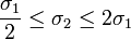 ). The table below illustrates the differences in the statistical inference in each of these situations. This table uses the following notation:
- Indexes 1 and 2 denote group one and group two, respectively
- T is the test statistics
- S is the standard error of the difference between two means
- df = degrees of freedom
- n1 and n2 are the number of observations in each group.
| Design | Sample Size | ||
|---|---|---|---|
| Equal | Unequal (different) | ||
| Population Variance | Equivalent |
|
|
| Non-equivalent (different) |
| ||
 where
where
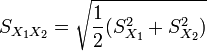 is the
 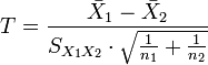 , where
 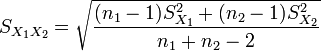 is an estimator of the common standard deviation of the two samples and df=n1 + n2 − 2
 , where
 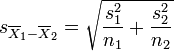 (not a pooled variance),
 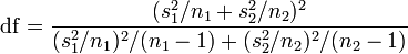 , which is called the
 Effect-Sizes
Effect size refers to a statistic calculated from a sample of data and are most commonly estimated with their corresponding errors. Sample-driven estimates of effect sizes are different from test statistics used in hypothesis testing as the former evaluate the strength of an apparent relationship and the latter assign a significance level reflecting whether the relationship could be due to chance. The effect size does not determine the significance level, or vice-versa. Given a large enough sample size, a statistical comparison will always show a significant difference unless the population effect size is trivial (i.e., zero). For example, a sample Pearson correlation coefficient of 0.1 would be strongly statistically significant when the sample size is 1000, but would be insignificant if the sample size is just 10. Reporting only the significant p-value from this analysis could be misleading if a correlation of 0.1 is too small to be of interest in a particular application.
Cohen's d
Cohen's d is the normalized difference between two means, i.e., the difference of means divided by a standard deviation for the data, i.e.,
- \(d = \frac{\bar{x}_1 - \bar{x}_2}{s}\).
Cohen's d is frequently used in estimating sample sizes.
- A lower Cohen's d indicates the necessity of larger sample sizes, i.e., need to have larger cohorts to be able to assess/detect if there are between-group differences in the observed data.
- The standard deviation \(s\) represents the population standard deviation (assuming the groups have approximately the same variances).
- \(s = \sqrt{\frac{(n_1-1)s^2_1 + (n_2-1)s^2_2}{n_1+n_2-2}}\), where
- \(s_1^2 = \frac{1}{n_1-1} \sum_{i=1}^{n_1} (x_{1,i} - \bar{x}_1)^2\) and \(s_2^2 = \frac{1}{n_2-1} \sum_{i=1}^{n_2} (x_{2,i} - \bar{x}_2)^2\).
This is referred to as the maximum likelihood estimator "Cohen's d", and it is related to Hedges's g by a scaling factor.
- Example: observing the heights of male and female visitors in England, the data (Aaron,Kromrey,& Ferron, 1998, November from a 2004 UK representative sample of 2436 men and 3311 women): Men: mean height = 1.75m; standard deviation = 89.9mm, and Women: mean height = 1.61m; standard deviation = 69.0mm. The effect size (using Cohen's d) would equal 1.72 (95% confidence interval: 1.66 – 1.78). This effect-size is large indicating that there is a consistent height difference, on average, between men and women visiting England.
Problems
- SOCR Home page: http://www.socr.ucla.edu
Translate this page:
