AP Statistics Curriculum 2007 Limits CLT
From Socr
(→ General Advance-Placement (AP) Statistics Curriculum - The Central Limit Theorem) |
m |
||
| Line 13: | Line 13: | ||
You can see [[SOCR_EduMaterials_Activities_GCLT_Applications | a number of applications of the Central Limit Theorem here]]. | You can see [[SOCR_EduMaterials_Activities_GCLT_Applications | a number of applications of the Central Limit Theorem here]]. | ||
| - | === | + | === General Statement of the Central Limit Theorem=== |
The Central Limit Theorem (CLT) argues that the distribution of the sum or average of independent observations from the same random process (with final mean and variance), will be approximately Normally distributed (i.e., bell-shaped curve). That is, the CLT express the fact that any sum or average of (many) independent and identically-distributed random variables will tend to be distributed according to a particular ''Attractor Distribution''; the Normal Distribution effectively represents the core of the universe of all (nice) distributions. | The Central Limit Theorem (CLT) argues that the distribution of the sum or average of independent observations from the same random process (with final mean and variance), will be approximately Normally distributed (i.e., bell-shaped curve). That is, the CLT express the fact that any sum or average of (many) independent and identically-distributed random variables will tend to be distributed according to a particular ''Attractor Distribution''; the Normal Distribution effectively represents the core of the universe of all (nice) distributions. | ||
| - | === | + | ===Symbolic Statement of the Central Limit Theorem=== |
The [http://en.wikipedia.org/wiki/Central_limit_theorem formal statement of the CLT is described here], however a more appropriate statement for many undergraduate and graduate classes use the following statement of the central limit theorem: | The [http://en.wikipedia.org/wiki/Central_limit_theorem formal statement of the CLT is described here], however a more appropriate statement for many undergraduate and graduate classes use the following statement of the central limit theorem: | ||
Revision as of 22:28, 18 March 2008
Contents |
General Advance-Placement (AP) Statistics Curriculum - The Central Limit Theorem
Motivation
The following example motivates the need to study the sampling distribution of the sample average, i.e., the distribution of 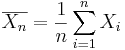 , as we vary the sample {
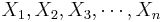 }.
}.
Suppose there are 10 world renowned laboratories, each is charged with conducting the same experiment (e.g., sequencing the genome Drosophila, the fruit fly), using the same protocols. One of the outcomes of this study that the sponsor agency is interested could be the average rate of occurrence of the ATC codon in 10,000 base-pairs in the Drosophila genome. After completing the sequencing of the genome, each lab selects a random segment of 1,000,000 base-pairs and counts the number of ATC codons in every segment of 10,000 base-pairs (there are 100 such segments). Finally they compute the average of the 100 counts they obtained. The funding/sponsoring agency receives 10 average counts from the 10 distinct laboratories. Most likely there will be differences between these averages.
The funding agency poses the most important question: Can we predict how much variation (i.e., discrepancy) there will be among the 10 lab averages, if we had only been able to fund/conduct 1 experiment at one site (due to resource/budgetary limitations)? In other words, if the sponsoring organization could only support one lab to carry out the experiment, can they estimate what are the possible errors that may be committed by using the sample average (of 100 samples) obtained from the chosen lab?
The answer is yes. They can accurately estimate the real count of ATC codons in the Drosophila genome from a single lab experiment as the sampling distribution of the average (across labs) is known to be (approximately) Normal!
You can see a number of applications of the Central Limit Theorem here.
General Statement of the Central Limit Theorem
The Central Limit Theorem (CLT) argues that the distribution of the sum or average of independent observations from the same random process (with final mean and variance), will be approximately Normally distributed (i.e., bell-shaped curve). That is, the CLT express the fact that any sum or average of (many) independent and identically-distributed random variables will tend to be distributed according to a particular Attractor Distribution; the Normal Distribution effectively represents the core of the universe of all (nice) distributions.
Symbolic Statement of the Central Limit Theorem
The formal statement of the CLT is described here, however a more appropriate statement for many undergraduate and graduate classes use the following statement of the central limit theorem:
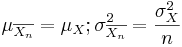
Let {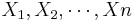 } be a random sample (IID) from a (native) distribution with well-defined and finite mean μX and variance
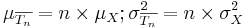
  . Then as n increases, the sampling distributions of the sample average and the total sum
 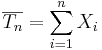 approach Normal distributions with corresponding means and variances:
In essence, the CLT implies that the Normal Distribution is the center of the universe of all nice distributions. This is the reason why we encounter frequent estimates involving arithmetic-averaging –- the pathway from a nice distribution to Normal distribution is paved by sample averages. In other words, the CLT provides a unifying framework for all (nice) distributions, the way the Grand Unifying Theory attempts to unite the theory behind the three fundamental forces in physics.
Are There CLTs for Other Sample Statistics?
The ramifications of the CLT go beyond the scope of this interpretation.
For example, one frequently wonders if there are other types of population-parameters or sample-statistics that yield similar limiting behavior.
- How large does the sample size have to be to ensure normality of the sample average or total sum?
- Does the convergence depend on the characteristics of the native distribution (e.g., shape, center, dispersion)?
- How about weighted averages, non-linear combinations or more general functions of the random sample?
Many other interesting questions are frequently asked by people exposed to the CLT. Some may have known theoretical answers (exact or approximate); other questions may be better addressed empirically by simulations and experiments (See the SOCR CLT Applet with Activity).
CLT Applications
A number of applications of the Central Limit Theorem are included in the SOCR CLT Activity.
To start the SOCR CLT Experiment
- Go to SOCR Experiments
- Select the SOCR Sampling Distribution CLT Experiment from the drop-down list of experiments in the left panel. The image below shows the interface to this experiment. Notice the main control widgets on this image (boxed in blue and pointed to by arrows). The generic control buttons on the top allow you to do one or multiple steps/runs, stop and reset this experiment. The two tabs in the main frame provide graphical access to the results of the experiment (Histograms and Summaries) or the Distribution selection panel (Distributions). Remember that choosing sample-sizes <= 16 will animate the samples (second graphing row), whereas larger sample-sizes (N>20) will only show the updates of the sampling distributions (bottom two graphing rows).

References
- SOCR Home page: http://www.socr.ucla.edu
Translate this page:
