AP Statistics Curriculum 2007 NonParam 2MedianPair
From Socr
Contents |
General Advance-Placement (AP) Statistics Curriculum - Differences of Medians of Two Paired Samples
Distribution-free (or non-parametric) statistical methods provide alternative to the (standard) parametric tests that we saw earlier, and are applicable when the distribution of the data is unknown.
Motivational Clinical Example
Whitley and Ball reported on the relative risk of mortality from 16 studies of septic patients. The outcome measure of interest was whether the patients developed complications of acute renal failure. The relative risk calculated in each study compared the risk of dying between patients with and without renal failure. A relative risk of 1.0 means no effect, and relative risk  suggests beneficial or detrimental effect of developing acute renal failure in sepsis. The main goal of the study was to determine whether developing acute renal failure as a complication of sepsis impacts patient mortality from the cumulative evidence in these 16 studies. The data of this study is included below.
| Study | Relative Risk | Sign (Relative Risk - 1) |
| 1 | 0.75 | - |
| 2 | 2.03 | + |
| 3 | 2.29 | + |
| 4 | 2.11 | + |
| 5 | 0.80 | - |
| 6 | 1.50 | + |
| 7 | 0.79 | - |
| 8 | 1.01 | + |
| 9 | 1.23 | + |
| 10 | 1.48 | + |
| 11 | 2.45 | + |
| 12 | 1.02 | + |
| 13 | 1.03 | + |
| 14 | 1.30 | + |
| 15 | 1.54 | + |
| 16 | 1.27 | + |
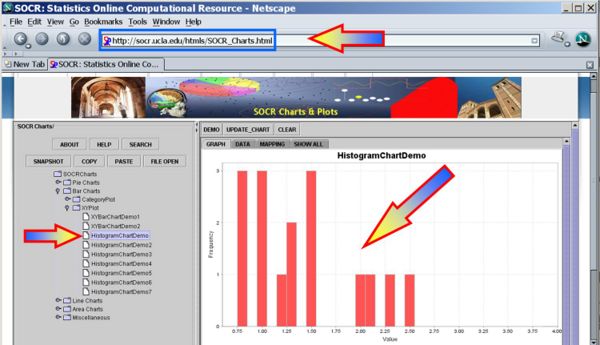
We see the clear analogy of this study design to the Paired or One-Sample studies we saw before. However, if we were to plot these data (Relative Risk), we can see that their distribution is hardly symmetric, unimodal and bell-shaped (i.e., not Normal). Therefore, we cannot use the Paired T-test to test a Null-Hypothesis that the mean Relative Risk is 1 using this parametric test.
The Sign-Test
The Sign Test is a non-parametric alternative to the One-Sample and Paired T-Test. The Sign Test has no requirements for the data to be Normally distributed. It assigns a positive (+) or negative (-) sign to each observation according to whether it is greater or less than some hypothesized value. It measures the difference between the  signs and how distinct the difference is from our expectations to observe by chance alone. For example, if there were no effects of developing acute renal failure on the outcome from sepsis, about half of the 16 studies above would be expected to have a relative risk less than 1.0 (a "-" sign) and the remaining 8 would be expected to have a relative risk greater than 1.0 (a "+" sign). In the actual data, 3 studies had "-" signs and the remaining 13 studies had "+" signs. Intuitively, this difference of 10 appears large to be simply due to random variation. If so, the effect of developing acute renal failure would be significant on the outcome from sepsis.
Calculations
Suppose N+ is the number of "+" signs and we fix a significance level of α = 0.05. And consider the following two hypotheses:
- Ho:N + = 8 (equivalent to N − = 8): The effect of developing acute renal failure is not significant on the outcome from sepsis.
-
 : The effect of developing acute renal failure is significant on the outcome from sepsis.
Define the following test-statistics
- Bs = max(N + ,N − ), where N + and N − are the number of positive and negative signs, respectively.
Then the distribution of  .
.
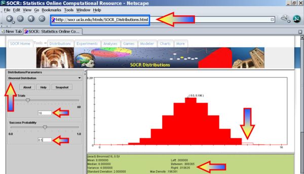
For our data, Bs = max(N + ,N − ) = max13,3 = 13 and the probability that such binomial variable exceeds 13 is P(Bin(16,0.5,13)) = 0.010635. Therefore, we can reject the null hypothesis Ho and regard as the significant effect of developing acute renal failure on the outcome from sepsis.
The Sign Test Using SOCR Analyses
It is much quicker to use SOCR Analyses to compute the statistical significance of the sign test. This SOCR Sign Test Activity may also be helpful in understanding how to use the sign test method in SOCR.
Example
A set of 12 identical twins is given psychological tests to determine whether the first born of the set tends to be more aggressive than the second born. Each twin is scored according to aggressiveness; a higher score indicates greater aggressiveness. Because of the natural pairing in a set of twins these data can be considered paired.
| Twin-Index | 1st Born | 2nd Born | Sign |
| 1 | 86 | 88 | - |
| 2 | 71 | 77 | - |
| 3 | 77 | 76 | + |
| 4 | 68 | 64 | + |
| 5 | 91 | 96 | - |
| 6 | 72 | 72 | 0 (Drop) |
| 7 | 77 | 65 | + |
| 8 | 91 | 90 | + |
| 9 | 70 | 65 | + |
| 10 | 71 | 80 | - |
| 11 | 88 | 81 | + |
| 12 | 87 | 72 | + |
We first plot the data using the SOCR Line Chart. Visually there does not seem to be a strong effect of the order of birth on baby's aggression.
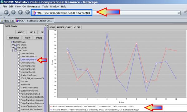
Next, we can use the SOCR Sign Test Analysis to quantitatively evaluate the evidence to reject the null hypothesis that there is no birth-order effect on baby's aggressiveness.
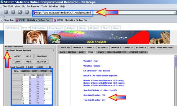
Clearly the p-value reported is 0.274, and our data can not reject the null hypothesis.
The Wilcoxon Signed Rank Test
Like the Sign Test and the T-Test, the Wilcoxon Signed Rank Test involves comparisons of differences between measurements. It requires that the data are measured at an interval level of measurement, but does not require assumptions about the form of the distribution of the measurements. It should therefore be used whenever the distributional assumptions of the T-Test are not satisfied.
Example
Whitley and Ball reported data on the central venous oxygen saturation (SvO2 (%)) from 10 consecutive patients at 2 time points; at admission and 6 hours after admission to the intensive care unit (ICU). The null hypothesis is that there is no effect of 6 hours of ICU treatment on SvO2. Under the null hypothesis, the mean of the differences between SvO2 at admission and that at 6 hours after admission should be zero.
| Patient | On Admission | At 6 Hours | Difference | Rank |
| 2 | 59.1 | 56.7 | -2.4 | 1 |
| 7 | 58.2 | 60.7 | 2.5 | 2 |
| 9 | 56.0 | 59.5 | 3.5 | 3 |
| 10 | 65.3 | 59.8 | -5.5 | 4 |
| 3 | 56.1 | 61.9 | 5.8 | 5 |
| 5 | 60.6 | 67.7 | 7.1 | 6 |
| 6 | 37.8 | 50.0 | 12.2 | 7 |
| 1 | 39.7 | 52.9 | 13.2 | 8 |
| 4 | 57.7 | 71.4 | 13.7 | 9 |
| 8 | 33.6 | 51.3 | 17.7 | 10 |
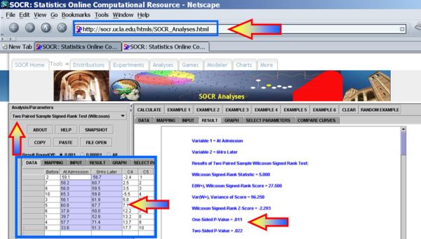
Clearly, we can reject the null-hypothesis at α = 0.05, as the one- and two-sided alternative hypotheses p-values for the Wilcoxon Signed Rank Test reported by the SOCR Analysis are respectively
- One-Sided p-value = 0.011
- Two-Sided p-value = 0.022
Result interpretation
The Results tab of the SOCR Wilcoxon signed-rank test applet contains the following output (this is for the data data above, and will change for other datasets, accordingly):
- Variable 1 = At_Admission
- Variable 2 = 6_Hrs_Later
- Results of Two Paired Sample Wilcoxon Signed Rank Test:
- Wilcoxon Signed-Rank Statistic = 5.000
- E(W+), Wilcoxon Signed-Rank Score = 27.500
- Var(W+), Variance of Score = 96.250
- Wilcoxon Signed-Rank Z-Score = -2.293
- One-Sided P-Value = .011
- Two-Sided P-Value = .022
Where:
- WStat, Wilcoxon Signed-Rank Statistic = data-driven estimate of the Wilcoxon Signed-Rank Statistic
- DataCase[] combo = QSortAlgorithm.rankList(diffListAbs);
- double wStat = 0;
- int lenList = combo.length;
- for (int i = 0; i < lenList; i++)
- if ( combo[i].getSign() ) wStat = wStat + combo[i].getRank();
- E(W+), Wilcoxon Signed-Rank Score = expectation of the Wilcoxon Signed-Rank Statistic, see page 414 Rice book (Mathematical Statistics and Data Analysis, 2dn Edition, by John Rice, Duxbury 1995.)
- Var(W+), Variance of Score = variance of the Wilcoxon Signed-Rank Statistic, see page 414 Rice book (Mathematical Statistics and Data Analysis, 2dn Edition, by John Rice, Duxbury 1995.)
- Wilcoxon Signed-Rank Z-Score =

- One-Sided P-Value = the one-sided (uni-directional) probability value expressing the strength of the evidence in the data to reject the null hypothesis that the two populations have the same medians (based on Gaussian, standard Normal, distribution).
- Two-Sided P-Value = the double-sided (non-directional) probability value expressing the strength of the evidence in the data to reject the null hypothesis that the two populations have the same medians (based on Gaussian, standard Normal, distribution).
Practice Problems
Treatment in Rats
Suppose 10 randomly selected rats were chosen to see if they could be trained to escape a maze. The rats were released and timed (seconds) before and after 2 weeks of training (N means the rat did not complete the maze-test). Do the data provide evidence to suggest that the escape time of rats is different after 2 weeks of training? Test using α = 0.05.
| Rat | Before | After | Sign |
| 1 | 100 | 50 | + |
| 2 | 38 | 12 | + |
| 3 | N | 45 | + |
| 4 | 122 | 62 | + |
| 5 | 95 | 90 | + |
| 6 | 116 | 100 | + |
| 7 | 56 | 75 | - |
| 8 | 135 | 52 | + |
| 9 | 104 | 44 | + |
| 10 | N | 50 | + |
Comparison and Validation of Automated Brain Volume Segmentation Methods
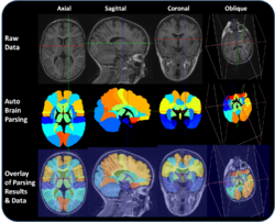
Automated brain volume segmentation is an important step in many modern computational brain mapping studies. Suppose we have two separate and competing versions of automated brain parsing (segmentation) algorithms that automatically tessellate (partition) the brain into 57 separate regions of interest (ROI's). An important question then is how consistent are these 2 different techniques, across the 57 ROIs. We can use the ROI volume as a measure of the resulting automated brain parcellation and compare the paired differences between the 2 methods across all ROIs. The image shows an example of a brain parcellated into these 57 regions and the table below contains the volumes of the 57 ROIs for the 2 different brain tessellation techniques. Use appropriate SOCR Analyses and relevant SOCR Charts to argue whether or not the 2 different methods are consistent and agree on their ROI labels.
| Index | Volume_Intensity | ROI_Name | Method1_Volume | Method2_Volume |
|---|---|---|---|---|
| 1 | 0 | Background | 9236455 | 9241667 |
| 2 | 21 | L_superior_frontal_gyrus | 78874 | 78693 |
| 3 | 22 | R_superior_frontal_gyrus | 69575 | 74391 |
| 4 | 23 | L_middle_frontal_gyrus | 67336 | 68872 |
| 5 | 24 | R_middle_frontal_gyrus | 68344 | 67024 |
| 6 | 25 | L_inferior_frontal_gyrus | 31912 | 21479 |
| 7 | 26 | R_inferior_frontal_gyrus | 26264 | 29035 |
| 8 | 27 | L_precentral_gyrus | 28942 | 33584 |
| 9 | 28 | R_precentral_gyrus | 35192 | 30537 |
| 10 | 29 | L_middle_orbitofrontal_gyrus | 10141 | 11608 |
| 11 | 30 | R_middle_orbitofrontal_gyrus | 9142 | 11850 |
| 12 | 31 | L_lateral_orbitofrontal_gyrus | 7164 | 5382 |
| 13 | 32 | R_lateral_orbitofrontal_gyrus | 5964 | 4947 |
| 14 | 33 | L_gyrus_rectus | 3840 | 1995 |
| 15 | 34 | R_gyrus_rectus | 2672 | 2994 |
| 16 | 41 | L_postcentral_gyrus | 24586 | 27672 |
| 17 | 42 | R_postcentral_gyrus | 21736 | 28159 |
| 18 | 43 | L_superior_parietal_gyrus | 25791 | 27500 |
| 19 | 44 | R_superior_parietal_gyrus | 28850 | 32674 |
| 20 | 45 | L_supramarginal_gyrus | 16445 | 22373 |
| 21 | 46 | R_supramarginal_gyrus | 11893 | 11018 |
| 22 | 47 | L_angular_gyrus | 20740 | 22245 |
| 23 | 48 | R_angular_gyrus | 20247 | 17793 |
| 24 | 49 | L_precuneus | 14491 | 12983 |
| 25 | 50 | R_precuneus | 15589 | 16323 |
| 26 | 61 | L_superior_occipital_gyrus | 6842 | 6106 |
| 27 | 62 | R_superior_occipital_gyrus | 5673 | 6539 |
| 28 | 63 | L_middle_occipital_gyrus | 15011 | 19085 |
| 29 | 64 | R_middle_occipital_gyrus | 19063 | 25747 |
| 30 | 65 | L_inferior_occipital_gyrus | 10411 | 8675 |
| 31 | 66 | R_inferior_occipital_gyrus | 12142 | 12277 |
| 32 | 67 | L_cuneus | 6935 | 9700 |
| 33 | 68 | R_cuneus | 7491 | 11765 |
| 34 | 81 | L_superior_temporal_gyrus | 29962 | 34934 |
| 35 | 82 | R_superior_temporal_gyrus | 30630 | 28788 |
| 36 | 83 | L_middle_temporal_gyrus | 27558 | 19633 |
| 37 | 84 | R_middle_temporal_gyrus | 26314 | 25301 |
| 38 | 85 | L_inferior_temporal_gyrus | 24817 | 24885 |
| 39 | 86 | R_inferior_temporal_gyrus | 25088 | 20661 |
| 40 | 87 | L_parahippocampal_gyrus | 6761 | 6977 |
| 41 | 88 | R_parahippocampal_gyrus | 6529 | 7964 |
| 42 | 89 | L_lingual_gyrus | 16752 | 14748 |
| 43 | 90 | R_lingual_gyrus | 20914 | 18500 |
| 44 | 91 | L_fusiform_gyrus | 16565 | 15020 |
| 45 | 92 | R_fusiform_gyrus | 14409 | 17311 |
| 46 | 101 | L_insular_cortex | 10779 | 9814 |
| 47 | 102 | R_insular_cortex | 8222 | 5599 |
| 48 | 121 | L_cingulate_gyrus | 14662 | 12490 |
| 49 | 122 | R_cingulate_gyrus | 16595 | 14489 |
| 50 | 161 | L_caudate | 1906 | 1608 |
| 51 | 162 | R_caudate | 2353 | 1997 |
| 52 | 163 | L_putamen | 3015 | 2622 |
| 53 | 164 | R_putamen | 2177 | 3758 |
| 54 | 165 | L_hippocampus | 3791 | 4454 |
| 55 | 166 | R_hippocampus | 3596 | 4673 |
| 56 | 181 | cerebellum | 174045 | 158617 |
| 57 | 182 | brainstem | 32567 | 28225 |
Moths Memory acquired at the Caterpillar Stage
References
- Whitley, E. and Ball, J. (2002) Statistics review 6: Nonparametric methods. Critical Care, 6(6): 509–513.
- SOCR Home page: http://www.socr.ucla.edu
Translate this page:
