AP Statistics Curriculum 2007 Normal Prob
From Socr
(→ General Advance-Placement (AP) Statistics Curriculum - Nonstandard Normal Distribution & Experiments: Finding Probabilities) |
|||
| Line 14: | Line 14: | ||
* See the special case of [[AP_Statistics_Curriculum_2007#The_Standard_Normal_Distribution | Standard Normal distribution]] where the mean is set to zero and a variance to one. | * See the special case of [[AP_Statistics_Curriculum_2007#The_Standard_Normal_Distribution | Standard Normal distribution]] where the mean is set to zero and a variance to one. | ||
| - | * The relation between the Standard and the General Normal distribution is provided by these simple linear transformations (Supposed X denotes General and Z denotes Standard Normal random variables): | + | * The relation between the Standard and the General Normal distribution is provided by these simple linear transformations (Supposed ''X'' denotes General and ''Z'' denotes Standard Normal random variables): |
: <math>Z = {X-\mu \over \sigma}</math> converts general normal scores to standard (Z) values. | : <math>Z = {X-\mu \over \sigma}</math> converts general normal scores to standard (Z) values. | ||
: <math>X = \mu +Z\sigma</math> converts standard scores to general normal values. | : <math>X = \mu +Z\sigma</math> converts standard scores to general normal values. | ||
| - | === | + | ===Examples=== |
| - | + | This [[Help_pages_for_SOCR_Distributions | Distributions help-page may be useful in understanding SOCR Distribution Applet]]. | |
| - | + | ====Systolic Arterial Pressure Example==== | |
| + | Suppose that the average systolic blood pressure (SBP) for a Los Angeles freeway commuter follows a Normal distribution with mean 130 mmHg and standard deviation 20 mmHg. Denote ''X'' to be the random variable representing the SBP measure for a randomly chosen commuter. Then <math>X\sim N(\mu=130, \sigma^2 =20^2)</math>. | ||
| - | * | + | * Find the percentage of LA freeway commuters that have a SBP less than 100. That is compute the following probability: ''p=P(X<100)=?'' (p=0.066776) |
| - | <center>[[Image: | + | <center>[[Image:SOCR_EBook_Dinov_RV_Normal_013108_Fig7.jpg|500px]]</center> |
| - | * | + | |
| - | <center>[[Image: | + | * If ''normal SBP'' is defined by the range [110 ; 140], and we take a random sample of 1,000 commuters and measure their SBP, how many would be expected to have ''normal SBP''? (Number = 1,000P(110<X<140)= 1,000*0.532807=532.807). |
| - | * | + | <center>[[Image:SOCR_EBook_Dinov_RV_Normal_013108_Fig8.jpg|500px]]</center> |
| - | <center>[[Image: | + | |
| - | * | + | * What is the 90<sup>th</sup> percentile for the SBP? That is what is <math>x_o</math>, so that <math>P(X<x_o)=0.9</math>? |
| - | < | + | <center>[[Image:SOCR_EBook_Dinov_RV_Normal_013108_Fig9.jpg|500px]]</center> |
| - | + | ||
| - | <center>[[Image: | + | * What is the range of SBP values that contain the central 80% of the SBPs for all commuters? That is what are <math>x_o, x_1</math>, so that <math>P(x_0<X<x_1)=0.8</math> and <math>{x_o+x_1\over2}=\mu=130</math> (i.e., they are symmetric around the mean)? (<math>x_o=104, x_1=156</math>) |
| + | <center>[[Image:SOCR_EBook_Dinov_RV_Normal_013108_Fig10.jpg|500px]]</center> | ||
<hr> | <hr> | ||
Revision as of 22:17, 31 January 2008
Contents |
General Advance-Placement (AP) Statistics Curriculum - Nonstandard Normal Distribution & Experiments: Finding Probabilities
Due to the Central Limit Theorem, the normal distribution is perhaps the most important model for studying various quantitative phenomena. Many numerical measurements (e.g., weight, time, etc.) can be well approximated by the normal distribution. While the mechanisms underlying natural processes may often be unknown, the use of the normal model can be theoretically justified by assuming that many small, independent effects are additively contributing to each observation.
General Normal Distribution
The (general) normal distribution is a continuous distribution that has similar exact areas, bound in terms of its mean, like the Standard Normal distribution and the x-axis on the symmetric intervals around the origin:
- The area: μ − σ < x < μ + σ = 0.8413 − 0.1587 = 0.6826
- The area: μ − 2σ < x < μ + 2σ = 0.9772 − 0.0228 = 0.9544
- The area: μ − 3σ < x < μ + 3σ = 0.9987 − 0.0013 = 0.9974

- General Normal density function
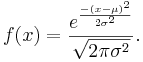
- See the special case of Standard Normal distribution where the mean is set to zero and a variance to one.
- The relation between the Standard and the General Normal distribution is provided by these simple linear transformations (Supposed X denotes General and Z denotes Standard Normal random variables):
-
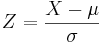 converts general normal scores to standard (Z) values.
- X = μ + Zσ converts standard scores to general normal values.
Examples
This Distributions help-page may be useful in understanding SOCR Distribution Applet.
Systolic Arterial Pressure Example
Suppose that the average systolic blood pressure (SBP) for a Los Angeles freeway commuter follows a Normal distribution with mean 130 mmHg and standard deviation 20 mmHg. Denote X to be the random variable representing the SBP measure for a randomly chosen commuter. Then 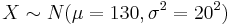 .
.
- Find the percentage of LA freeway commuters that have a SBP less than 100. That is compute the following probability: p=P(X<100)=? (p=0.066776)

- If normal SBP is defined by the range [110 ; 140], and we take a random sample of 1,000 commuters and measure their SBP, how many would be expected to have normal SBP? (Number = 1,000P(110<X<140)= 1,000*0.532807=532.807).

- What is the 90th percentile for the SBP? That is what is xo, so that P(X < xo) = 0.9?

- What is the range of SBP values that contain the central 80% of the SBPs for all commuters? That is what are xo,x1, so that P(x0 < X < x1) = 0.8 and
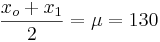 (i.e., they are symmetric around the mean)? (xo = 104,x1 = 156)

References
- SOCR Home page: http://www.socr.ucla.edu
Translate this page:
