AP Statistics Curriculum 2007 Normal Std
From Socr
| Line 1: | Line 1: | ||
| - | + | ==[[AP_Statistics_Curriculum_2007 | General Advance-Placement (AP) Statistics Curriculum]] - Standard Normal Variables and Experiments== | |
| - | + | ||
| - | + | ||
| - | + | ||
| - | + | ||
| - | + | ||
| - | + | ||
| - | + | ||
| - | + | ||
| - | + | ||
| - | + | ||
| - | + | ||
| - | + | ||
| - | + | ||
| - | + | ||
| - | + | ||
| - | + | ||
| - | + | ||
| - | + | ||
| - | + | ||
| - | + | ||
| - | + | ||
| - | + | ||
| - | + | ||
| - | + | ||
| - | + | ||
| - | + | ||
| - | + | ||
| - | + | ||
| - | + | ||
| - | + | ||
| - | + | ||
| - | + | ||
| - | + | ||
=== Standard Normal Distribution=== | === Standard Normal Distribution=== | ||
Revision as of 20:18, 31 January 2008
Contents |
General Advance-Placement (AP) Statistics Curriculum - Standard Normal Variables and Experiments
Standard Normal Distribution
The standard normal distribution is a continuous distribution where the following exact areas are bound between the Standard Normal Density function and the x-axis on the symmetric intervals around the origin:
- The area: -1 < z < 1 = 0.8413 - 0.1587 = 0.6826
- The area: -2.0 < z < 2.0 = 0.9772 - 0.0228 = 0.9544
- The area: -3.0 < z < 3.0 = 0.9987 - 0.0013 = 0.9974

- Standard Normal density function
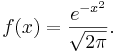
- The Standard Normal distribution is also a special case of the more general normal distribution where the mean is set to zero and a variance to one. The Standard Normal distribution is often called the bell curve because the graph of its probability density resembles a bell.
Experiments
Suppose we decide to test the state of 100 used batteries. To do that, we connect each battery to a volt-meter by randomly attaching the positive (+) and negative (-) battery terminals to the corresponding volt-meter's connections. Electrical current always flows from + to -, i.e., the current goes in the direction of the voltage drop. Depending upon which way the battery is connected to the volt-meter we can observe positive or negative voltage recordings (voltage is just a difference, which forces current to flow from higher to the lower voltage.) Denote Xi={measured voltage for battery i} - this is random variable 0 and assume the distribution of all Xi is Standard Normal,  . Use the Normal Distribution (with mean=0 and variance=1) in the SOCR Distribution applet to address the following questions. This Distributions help-page may be useful in understanding SOCR Distribution Applet. How many batteries, from the sample of 100, can we expect to have?
- Absolute Voltage > 1? P(X>1) = 0.1586, thus we expect 15-16 batteries to have voltage exceeding 1.

- |Absolute Voltage| > 1? P(|X|>1) = 1- 0.682689=0.3173, thus we expect 31-32 batteries to have absolute voltage exceeding 1.

- Voltage < -2? P(X<-2) = 0.0227, thus we expect 2-3 batteries to have voltage less than -2.

- Voltage <= -2? P(X<=-2) = 0.0227, thus we expect 2-3 batteries to have voltage less than or equal to -2.
- -1.7537 < Voltage < 0.8465? P(-1.7537 < X < 0.8465) = 0.761622, thus we expect 76 batteries to have voltage in this range.

References
- SOCR Home page: http://www.socr.ucla.edu
Translate this page:
