AP Statistics Curriculum 2007 Prob Basics
From Socr
(→A brief History) |
|||
| (23 intermediate revisions not shown) | |||
| Line 1: | Line 1: | ||
==[[AP_Statistics_Curriculum_2007 | General Advance-Placement (AP) Statistics Curriculum]] - Fundamentals of Probability Theory== | ==[[AP_Statistics_Curriculum_2007 | General Advance-Placement (AP) Statistics Curriculum]] - Fundamentals of Probability Theory== | ||
| + | |||
| + | === A brief History=== | ||
| + | Currently, there is no evidence that the ancient Greeks or the Romans had any interests or pursued the notion of predicting future likelihoods, probabilities, outcome chances, or odds. The first recorded attempts to develop a theory describing future events was driven by examining gambling games during hte early Renaissance. In 1550, an Italian polymath [https://en.wikipedia.org/wiki/Gerolamo_Cardano Gerolamo Cardano] (1501-1576) wrote a [https://books.google.com/books/about/Foundations_of_discrete_mathematics.html?id=xHlQAAAAMAAJ paper] addressing the chance of certain outcomes in rolls of dice, which presented the first definition of ''probability''. This manuscript was only in 1576 and then printed in 1663. | ||
| + | |||
| + | The next substantial contributions to probability theory was a [http://wiki.socr.umich.edu/images/b/bc/Probability_Expectation_Formulation_Pascal_Fermat_1654.pdf letter exchange] by [https://en.wikipedia.org/wiki/Blaise_Pascal Blaise Pascal] (1623-1662) and [https://en.wikipedia.org/wiki/Pierre_de_Fermat Pierre de Fermat] (1601-1665). Pascal and Fermat discussed a gambling problem proposed in 1654 by [https://fr.wikipedia.org/wiki/Antoine_Gombaud,_chevalier_de_M%C3%A9r%C3%A9 Chevalier de Mere], which examined the fundamentals of probability theory. The key question related to the number of experiments required to ensure obtaining a total sum of 6 when rolling two fair hexagonal dice. The letter correspondence between Pascal and Fermat led to the formulation of probability and expectation. | ||
| + | |||
| + | The most popular modern probability theory foundation (as there are many alternative axiomatic definitions) was laid out by [https://en.wikipedia.org/wiki/Andrey_Nikolaevich_Kolmogorov Andrey Kolmogorov], who defined the notion of ''sample space'' and proposed an axiomatic system for probability theory, and [https://en.wikipedia.org/wiki/Richard_von_Mises Richard von Mises], who tied in measure theory. | ||
=== Fundamentals of Probability Theory=== | === Fundamentals of Probability Theory=== | ||
| - | Probability theory plays role in all studies of natural processes across scientific disciplines. The need for a theoretical probabilistic foundation is obvious since natural variation | + | Probability theory plays a role in all studies of natural processes across scientific disciplines. The need for a theoretical probabilistic foundation is obvious since natural variation affects all measurements, observations and findings about different phenomena. Probability theory provides the basic techniques for statistical inference. |
===Random Sampling=== | ===Random Sampling=== | ||
A '''simple random sample''' of ''n'' items is a sample in which every member of the population has an equal chance of being selected ''and'' the members of the sample are chosen independently. | A '''simple random sample''' of ''n'' items is a sample in which every member of the population has an equal chance of being selected ''and'' the members of the sample are chosen independently. | ||
| - | * '''Example''': Consider a class of students as the population under study. If we select a sample of size 5, each possible sample of size 5 must have the same chance of being selected. When a sample is chosen randomly | + | * '''Example''': Consider a class of students as the population under study. If we select a sample of size 5, each possible sample of size 5 must have the same chance of being selected. When a sample is chosen randomly, the process of selection that is random. How could we select five members from this class randomly? Random sampling from finite (or countable) populations is well-defined. On the contrary, random sampling of uncountable populations is only allowed under the [http://en.wikipedia.org/wiki/Axiom_of_Choice Axiom of Choice]. |
* '''Random Number Generation''' using [[SOCR]]: You can use [http://socr.ucla.edu/htmls/SOCR_Modeler.html SOCR Modeler] to [[SOCR_EduMaterials_Activities_RNG | construct random samples]] of any size from a large number of distribution families. | * '''Random Number Generation''' using [[SOCR]]: You can use [http://socr.ucla.edu/htmls/SOCR_Modeler.html SOCR Modeler] to [[SOCR_EduMaterials_Activities_RNG | construct random samples]] of any size from a large number of distribution families. | ||
| Line 13: | Line 20: | ||
* '''Questions''': | * '''Questions''': | ||
**How would you go about randomly selecting five students from a class of 100? | **How would you go about randomly selecting five students from a class of 100? | ||
| - | **How | + | **How likely the sample is to represent of the population? The sample won’t exactly resemble the population as there will be some chance of variation. This discrepancy is called chance '''error due to sampling'''. |
| - | * '''Definition''': '''Sampling bias''' is non- | + | * '''Definition''': '''Sampling bias''' is non-random and refers to some members having a tendency to be selected more readily than others. When the sample is biased the statistics turn out to be poor estimates. |
===Hands-on activities=== | ===Hands-on activities=== | ||
| Line 22: | Line 29: | ||
** '''Swap''' strategy - choose one card first, as the computer reveals one of the donkey cards, you always swap your original guess and go with the third face-down card! | ** '''Swap''' strategy - choose one card first, as the computer reveals one of the donkey cards, you always swap your original guess and go with the third face-down card! | ||
| - | * You can try the [http://socr.ucla.edu/htmls/SOCR_Experiments.html Monty Hall Experiment] | + | * You can try the [http://socr.ucla.edu/htmls/SOCR_Experiments.html Monty Hall Experiment] as well. There you can run a very large number of trials automatically and observe the outcomes empirically. Notice that your chance to win doubles if you use the swap-strategy. Why is that? |
* See the [[SOCR_EduMaterials_Activities_MontyHall | SOCR Monty Hall Activity]]. | * See the [[SOCR_EduMaterials_Activities_MontyHall | SOCR Monty Hall Activity]]. | ||
| + | * See the [[AP_Statistics_Curriculum_2007_Prob_Rules#Monty_Hall_Problem | conditional probability derivation]] of the exact chance of success. | ||
===Law of Large Numbers=== | ===Law of Large Numbers=== | ||
| - | When studying the behavior of coin tosses, the law of large numbers implies that the relative proportion (relative frequency) of heads-to-tails in a coin toss experiment becomes more and more stable as the number of tosses increases. This regards the relative frequencies, not absolute counts of | + | When studying the behavior of coin tosses, the law of large numbers implies that the relative proportion (relative frequency) of heads-to-tails in a coin toss experiment becomes more and more stable as the number of tosses increases. This regards to the relative frequencies, not absolute counts of heads and tails. |
| - | * There are two widely held ''misconceptions'' about | + | * There are two widely held ''misconceptions'' about the law of large numbers relating to coin tosses: |
| - | **Differences between the actual numbers of heads | + | **Differences between the actual numbers of heads and tails become more variable with increase of the number of tosses – a sequence of 10 heads doesn’t increase the chances of selecting a tail on the next trial. |
** Coin toss results are independent and fair, and the outcome behavior is unpredictable. | ** Coin toss results are independent and fair, and the outcome behavior is unpredictable. | ||
| Line 62: | Line 70: | ||
* '''First axiom''': The probability of an event is a non-negative real number: <math>P(E)\geq 0</math>, <math>\forall E\subseteq S</math>, where <math>S</math> is the sample space. | * '''First axiom''': The probability of an event is a non-negative real number: <math>P(E)\geq 0</math>, <math>\forall E\subseteq S</math>, where <math>S</math> is the sample space. | ||
| - | * '''Second axiom''': This is the assumption of '''unit measure''': | + | * '''Second axiom''': This is the assumption of '''unit measure''': the probability that some elementary event in the entire sample space will occur is 1. More specifically, there are no elementary events outside the sample space: <math>P(S) = 1</math>. This is often overlooked in some mistaken probability calculations if you cannot precisely define the whole sample space, then the probability of any subset cannot be defined either. |
* '''Third axiom''': This is the assumption of additivity: Any countable sequence of pair-wise disjoint events <math>E_1, E_2, ...</math> satisfies <math>P(E_1 \cup E_2 \cup \cdots) = \sum_i P(E_i).</math> | * '''Third axiom''': This is the assumption of additivity: Any countable sequence of pair-wise disjoint events <math>E_1, E_2, ...</math> satisfies <math>P(E_1 \cup E_2 \cup \cdots) = \sum_i P(E_i).</math> | ||
| Line 69: | Line 77: | ||
===Birthday Paradox=== | ===Birthday Paradox=== | ||
| - | The [[SOCR_EduMaterials_Activities_BirthdayExperiment | Birthday Paradox]] provides an interesting illustration of some of the fundamental probability concepts. | + | The [[SOCR_EduMaterials_Activities_BirthdayExperiment | Birthday Paradox Experiment]] provides an interesting illustration of some of the fundamental probability concepts. |
In a random group of N people, what is the probability, P, that ''at least two people have the same birthday''? | In a random group of N people, what is the probability, P, that ''at least two people have the same birthday''? | ||
| Line 77: | Line 85: | ||
The reason for such high probability is that any of the 23 people can compare their birthday with any other one, not just you comparing your birthday to anybody else’s. | The reason for such high probability is that any of the 23 people can compare their birthday with any other one, not just you comparing your birthday to anybody else’s. | ||
| - | There are N-Choose-2 = 20*19/2 ways to select a pair | + | There are N-Choose-2 = 20*19/2 ways to select a pair of people from a group of 20. Assume there are 365 days in a year, P(one-particular-pair-same-B-day)=1/365, and |
P(one-particular-pair-failure)=1-1/365 ~ 0.99726. | P(one-particular-pair-failure)=1-1/365 ~ 0.99726. | ||
| - | For N=20, 20-Choose-2 = 190. E={No 2 people have the same birthday is the event all 190 pairs fail (have different birthdays)}, then P(E) = P(failure)190 = 0. | + | For N=20, 20-Choose-2 = 190. E={No 2 people have the same birthday is the event all 190 pairs fail (have different birthdays)}, then P(E) = P(failure)<sup>190</sup> = 0.99726<sup>190</sup> = 0.59. Hence, P(at-least-one-success)=1-0.59=0.41, quite high. |
Note: for N=42, P>0.9. | Note: for N=42, P>0.9. | ||
| + | |||
| + | This is an ''approximate solution'' to the Birthday problem. You can also see the ''exact solution'' in the [[SOCR_EduMaterials_Activities_BirthdayExperiment#Exact_Calculations | Birthday Paradox Activity]]. | ||
| + | |||
| + | ===Examples=== | ||
| + | ====Elementary Probability==== | ||
| + | Each of the three boxes below contains two types of balls (''Red'' and ''Green''). Box 1 has ''4 Red'' and ''3 Green'' balls, box 2 has ''3 Red'' and ''2 Green'' balls, and box 3 has ''2 Red'' and ''1 Green'' balls. All balls are identical except for their labels. Which of the three boxes do you most likely to draw a ''Red'' ball from? In other words, if a randomly drawn ball is known to be Red, which box is the one that we most likely draw the ball out of? | ||
| + | <center>[[Image:SOCR_EBook_Dinov_Prob_BallUrn_040308_Fig4.jpg|400px]]</center> | ||
| + | |||
| + | * ''Exact solution'': The probabilities of drawing a Red ball out of each of the 3 boxes are 4/7, 3/5 and 2/3, respectively. The smallest common denominator of the prime numbers 7, 5 and 3 is their product 105. Thus, these probabilities may also be expressed as 60/105, 63/105 and 70/105, respectively. Clearly, the highest chance of drawing a Red ball is associated with box 3, despite the fact that this box has the smallest number of Red balls. | ||
| + | |||
| + | * ''Empirical solution'': This problem may also be explored experimentally using the [http://socr.ucla.edu/htmls/exp/Ball_and_Urn_Experiment.html SOCR Ball-and-Urn Experiment] (see [[SOCR_EduMaterials_Activities_BallAndRunExperiment |this activity]]). Each of the 3 figures below illustrates this experiment, where we sample (''with replacement'') 100 balls from each box, respectively. | ||
| + | ** Box 1: To empirically test the chance of drawing a Red ball from box 1, we set N=7 (total number of balls), R=4 (number of red balls in the population, and n=100 (number of balls we sample, i.e., number of experiments we do). The result of these 100 random draws will vary each time. However one such experiment generated 62 Red balls out of the 100 draws (see image below and the value of the ''Y=62'' variable in the summary table). <center>[[Image:SOCR_EBook_Dinov_Prob_BallUrn_040308_Fig1.jpg|400px]]</center> | ||
| + | ** Box 2: Now we set N=5 (total number of balls), R=3 (number of red balls in the population, and n=100 (number of balls we sample, i.e., number of experiments we do). Again, the result of these 100 random draws will vary each time. However one such experiment generated 64 Red balls out of the 100 draws (see image below and the value of the variable ''Y=64'' in the summary table below the graph). <center>[[Image:SOCR_EBook_Dinov_Prob_BallUrn_040308_Fig2.jpg|400px]]</center> | ||
| + | ** Box 3: Finally, we can set N=3 (total number of balls), R=2 (number of red balls in the population, and n=100 (number of balls we sample, i.e., number of experiments we do). Again, the result of these 100 random draws will vary each time. However one such experiment generated 71 Red balls out of the 100 draws (see image below and the value of the variable ''Y=71'' in the summary table below the graph). | ||
| + | <center>[[Image:SOCR_EBook_Dinov_Prob_BallUrn_040308_Fig3.jpg|400px]]</center> | ||
| + | |||
| + | From these empirical tests, we can ''propose'' that a Red ball is most likely to be drawn from Box 3. Again, remember that these simulations will produce different results each time we do the experiments. However, the [[AP_Statistics_Curriculum_2007_Distrib_MeanVar | expected means]] (expected number of Red balls in sample of 100), which are reported in the bottom-right tables (for each box setting), indicate this conclusion more reliably. These expected Red ball counts for the 3 boxes are '''57.14''', '''60.0''' and '''66.67''', respectively. | ||
| + | |||
| + | ====SOCR Empirical Probabilities==== | ||
| + | For each of these hands-on interactive experiments discuss the sample space, probabilities, events of interest, event operations, and how to compute theoretically and empirically the probabilities of these events. | ||
| + | : [[SOCR_EduMaterials_Activities_BuffonCoinExperiment | Buffon Coin Experiment]] | ||
| + | : [[SOCR_EduMaterials_Activities_BuffonNeedleExperiment | Buffon Needle Experiment]] | ||
| + | : [[SOCR_EduMaterials_Activities_PokerDiceeriment | Poker Dice Experiment]] | ||
| + | : [[SOCR_EduMaterials_Activities_PokerExperiment | Poker Experiment]] | ||
| + | : [[SOCR_EduMaterials_Activities_SpinnerExperiment | Spinner Experiment]] | ||
| + | : Other [[SOCR_EduMaterials_ExperimentsActivities | experiments from this collection]]. | ||
| + | |||
| + | ===[[EBook_Problems_Prob_Basics |Problems]]=== | ||
<hr> | <hr> | ||
Current revision as of 13:16, 13 April 2018
Contents
|
General Advance-Placement (AP) Statistics Curriculum - Fundamentals of Probability Theory
A brief History
Currently, there is no evidence that the ancient Greeks or the Romans had any interests or pursued the notion of predicting future likelihoods, probabilities, outcome chances, or odds. The first recorded attempts to develop a theory describing future events was driven by examining gambling games during hte early Renaissance. In 1550, an Italian polymath Gerolamo Cardano (1501-1576) wrote a paper addressing the chance of certain outcomes in rolls of dice, which presented the first definition of probability. This manuscript was only in 1576 and then printed in 1663.
The next substantial contributions to probability theory was a letter exchange by Blaise Pascal (1623-1662) and Pierre de Fermat (1601-1665). Pascal and Fermat discussed a gambling problem proposed in 1654 by Chevalier de Mere, which examined the fundamentals of probability theory. The key question related to the number of experiments required to ensure obtaining a total sum of 6 when rolling two fair hexagonal dice. The letter correspondence between Pascal and Fermat led to the formulation of probability and expectation.
The most popular modern probability theory foundation (as there are many alternative axiomatic definitions) was laid out by Andrey Kolmogorov, who defined the notion of sample space and proposed an axiomatic system for probability theory, and Richard von Mises, who tied in measure theory.
Fundamentals of Probability Theory
Probability theory plays a role in all studies of natural processes across scientific disciplines. The need for a theoretical probabilistic foundation is obvious since natural variation affects all measurements, observations and findings about different phenomena. Probability theory provides the basic techniques for statistical inference.
Random Sampling
A simple random sample of n items is a sample in which every member of the population has an equal chance of being selected and the members of the sample are chosen independently.
- Example: Consider a class of students as the population under study. If we select a sample of size 5, each possible sample of size 5 must have the same chance of being selected. When a sample is chosen randomly, the process of selection that is random. How could we select five members from this class randomly? Random sampling from finite (or countable) populations is well-defined. On the contrary, random sampling of uncountable populations is only allowed under the Axiom of Choice.
- Random Number Generation using SOCR: You can use SOCR Modeler to construct random samples of any size from a large number of distribution families.
- Questions:
- How would you go about randomly selecting five students from a class of 100?
- How likely the sample is to represent of the population? The sample won’t exactly resemble the population as there will be some chance of variation. This discrepancy is called chance error due to sampling.
- Definition: Sampling bias is non-random and refers to some members having a tendency to be selected more readily than others. When the sample is biased the statistics turn out to be poor estimates.
Hands-on activities
- Monty Hall (Three-Door) Problem: Go to SOCR Games and select the Monty Hall Game. Click in the Information button to get the instructions on using the applet. Run the game 10 times with one of two strategies:
- Stay-home strategy - choose one card first, as the computer reveals one of the donkey cards, you always stay with the card you originally chose.
- Swap strategy - choose one card first, as the computer reveals one of the donkey cards, you always swap your original guess and go with the third face-down card!
- You can try the Monty Hall Experiment as well. There you can run a very large number of trials automatically and observe the outcomes empirically. Notice that your chance to win doubles if you use the swap-strategy. Why is that?
- See the SOCR Monty Hall Activity.
- See the conditional probability derivation of the exact chance of success.
Law of Large Numbers
When studying the behavior of coin tosses, the law of large numbers implies that the relative proportion (relative frequency) of heads-to-tails in a coin toss experiment becomes more and more stable as the number of tosses increases. This regards to the relative frequencies, not absolute counts of heads and tails.
- There are two widely held misconceptions about the law of large numbers relating to coin tosses:
- Differences between the actual numbers of heads and tails become more variable with increase of the number of tosses – a sequence of 10 heads doesn’t increase the chances of selecting a tail on the next trial.
- Coin toss results are independent and fair, and the outcome behavior is unpredictable.
Types of probabilities
Probability models have two essential components: sample space and probabilities.
- Sample space (S) for a random experiment is the set of all possible outcomes of the experiment.
- An event is a collection of outcomes.
- An event occurs if any outcome making up that event occurs.
- Probabilities for each event in the sample space.
Where do the outcomes and the probabilities come from?
- Probabilities may come from models – say mathematical/physical description of the sample space and the chance of each event. Construct a fair die tossing game.
- Probabilities may be derived from data – data observations determine our probability distribution. Say we toss a coin 100 times and the observed Head/Tail counts are used as probabilities.
- Subjective Probabilities – combining data and psychological factors to design a reasonable probability table (e.g., gambling, stock market).
Event Manipulations
Just like we develop rules for numeric arithmetic, we like to use certain event-manipulation rules (event-arithmetic).
- Complement: The complement of an event A, denoted Ac or A', occurs if and only if A does not occur.
-
 , read "A or B", contains all outcomes in A or B (or both).
-
 , read "A and B", contains all outcomes which are in both A and B.
- Draw Venn diagram pictures of these composite events.
- Mutually exclusive events cannot occur at the same time (
 ).
).
Axioms of probability
- First axiom: The probability of an event is a non-negative real number:
 ,
,  , where S is the sample space.
- Second axiom: This is the assumption of unit measure: the probability that some elementary event in the entire sample space will occur is 1. More specifically, there are no elementary events outside the sample space: P(S) = 1. This is often overlooked in some mistaken probability calculations if you cannot precisely define the whole sample space, then the probability of any subset cannot be defined either.
- Third axiom: This is the assumption of additivity: Any countable sequence of pair-wise disjoint events E1,E2,... satisfies
- Note: For a finite sample space, a sequence of number {
 } is a probability distribution for a sample space S = {
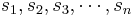 }, if the probability of the outcome sk, p(sk) = pk, for each
  , all
, all  and
and  .
.
Birthday Paradox
The Birthday Paradox Experiment provides an interesting illustration of some of the fundamental probability concepts.
In a random group of N people, what is the probability, P, that at least two people have the same birthday?
- Example, if N=23, P>0.5. Main confusion arises from the fact that in real life we rarely meet people having the same birthday as us, and we meet more than 23 people.
The reason for such high probability is that any of the 23 people can compare their birthday with any other one, not just you comparing your birthday to anybody else’s.
There are N-Choose-2 = 20*19/2 ways to select a pair of people from a group of 20. Assume there are 365 days in a year, P(one-particular-pair-same-B-day)=1/365, and P(one-particular-pair-failure)=1-1/365 ~ 0.99726.
For N=20, 20-Choose-2 = 190. E={No 2 people have the same birthday is the event all 190 pairs fail (have different birthdays)}, then P(E) = P(failure)190 = 0.99726190 = 0.59. Hence, P(at-least-one-success)=1-0.59=0.41, quite high. Note: for N=42, P>0.9.
This is an approximate solution to the Birthday problem. You can also see the exact solution in the Birthday Paradox Activity.
Examples
Elementary Probability
Each of the three boxes below contains two types of balls (Red and Green). Box 1 has 4 Red and 3 Green balls, box 2 has 3 Red and 2 Green balls, and box 3 has 2 Red and 1 Green balls. All balls are identical except for their labels. Which of the three boxes do you most likely to draw a Red ball from? In other words, if a randomly drawn ball is known to be Red, which box is the one that we most likely draw the ball out of?

- Exact solution: The probabilities of drawing a Red ball out of each of the 3 boxes are 4/7, 3/5 and 2/3, respectively. The smallest common denominator of the prime numbers 7, 5 and 3 is their product 105. Thus, these probabilities may also be expressed as 60/105, 63/105 and 70/105, respectively. Clearly, the highest chance of drawing a Red ball is associated with box 3, despite the fact that this box has the smallest number of Red balls.
- Empirical solution: This problem may also be explored experimentally using the SOCR Ball-and-Urn Experiment (see this activity). Each of the 3 figures below illustrates this experiment, where we sample (with replacement) 100 balls from each box, respectively.
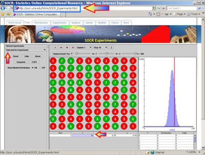
- Box 1: To empirically test the chance of drawing a Red ball from box 1, we set N=7 (total number of balls), R=4 (number of red balls in the population, and n=100 (number of balls we sample, i.e., number of experiments we do). The result of these 100 random draws will vary each time. However one such experiment generated 62 Red balls out of the 100 draws (see image below and the value of the Y=62 variable in the summary table).
- Box 2: Now we set N=5 (total number of balls), R=3 (number of red balls in the population, and n=100 (number of balls we sample, i.e., number of experiments we do). Again, the result of these 100 random draws will vary each time. However one such experiment generated 64 Red balls out of the 100 draws (see image below and the value of the variable Y=64 in the summary table below the graph).
- Box 3: Finally, we can set N=3 (total number of balls), R=2 (number of red balls in the population, and n=100 (number of balls we sample, i.e., number of experiments we do). Again, the result of these 100 random draws will vary each time. However one such experiment generated 71 Red balls out of the 100 draws (see image below and the value of the variable Y=71 in the summary table below the graph).
- Box 1: To empirically test the chance of drawing a Red ball from box 1, we set N=7 (total number of balls), R=4 (number of red balls in the population, and n=100 (number of balls we sample, i.e., number of experiments we do). The result of these 100 random draws will vary each time. However one such experiment generated 62 Red balls out of the 100 draws (see image below and the value of the Y=62 variable in the summary table).


From these empirical tests, we can propose that a Red ball is most likely to be drawn from Box 3. Again, remember that these simulations will produce different results each time we do the experiments. However, the expected means (expected number of Red balls in sample of 100), which are reported in the bottom-right tables (for each box setting), indicate this conclusion more reliably. These expected Red ball counts for the 3 boxes are 57.14, 60.0 and 66.67, respectively.
SOCR Empirical Probabilities
For each of these hands-on interactive experiments discuss the sample space, probabilities, events of interest, event operations, and how to compute theoretically and empirically the probabilities of these events.
- Buffon Coin Experiment
- Buffon Needle Experiment
- Poker Dice Experiment
- Poker Experiment
- Spinner Experiment
- Other experiments from this collection.
Problems
References
- SOCR Home page: http://www.socr.ucla.edu
Translate this page:
