AP Statistics Curriculum 2007 Prob Rules
From Socr
General Advance-Placement (AP) Statistics Curriculum - Probability Theory Rules
Addition Rule
Let's start with an example. Suppose the chance of colder weather (C) is 30%, chance of rain (R) and colder weather (C) is 15% and the chance of rain or colder weather is 75%. What is the chance of rain. This can be computed by observing that \(P(R) - P(R \cup C) + P(C) = P(R \cap C)\). Thus, \(P(R) = P(R \cup C) − P(C) + P(R \cap C)= 0.75 − 0.3 + 0.15 = 0.6\). How can this observation be generalized?
The probability of a union, also called the Inclusion-Exclusion principle allows us to compute probabilities of composite events represented as unions (i.e., sums) of simpler events.

For events A1, ..., An in a probability space (S,P), the probability of the union for n=2 is

For n=3,

In general, for any n,


Conditional Probability
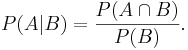
The conditional probability of A occurring given that B occurs is given by
Suppose X and Y are jointly continuous random variables with a joint density \(ƒ_{X,Y}(x,y)\). If A and B (non-trivial) are subsets of the ranges of X and Y (e.g., intervals), then:
- \( P(X \in A \mid Y \in B) = \frac{\int_{y\in B}\int_{x\in A} f_{X,Y}(x,y)\,dx\,dy}{\int_{y\in B}\int_{x\in\Omega} f_{X,Y}(x,y)\,dx\,dy}. \)
In the special case where B={y0}, representing a single point, the conditional probability is:
- \( P(X \in A \mid Y = y_0) = \frac{\int_{x\in A} f_{X,Y}(x,y_0)\,dx}{\int_{x\in\Omega} f_{X,Y}(x,y_0)\,dx}. \)
Of course, if the set (range) A is trivial, then the conditional probability is zero.
- See the example of the SOCR HTML5 Bivariate (2D) Normal Distribution Calculator (webapp).
- The conditional probability distribution of X given Y = \(y_0\), \(f_{X|Y=y_o}\), is given by:
- \( f_{X|y_o} \sim N \left ( \mu_{X|y_o} = \mu_X +\rho \frac{\sigma_X}{\sigma_Y}(y_o-\mu_Y), \sigma_{X|y_o}^2 = \sigma_X^2(1-\rho^2) \right) \), where
- \( X \sim N (\mu_X, \sigma_X^2) \),
- \( Y \sim N (\mu_Y, \sigma_Y^2) \), and
- \( \rho = Corr(X,Y)\) is the correlation between X and Y.
- This expression of the density assumes that the conditional mean of X given \(y_o\) is linear in y and the conditional variance of X given \(y_o\) is constant.
Examples
Contingency table
Here is the data of 400 Melanoma (skin cancer) Patients by Type and Site
| Type | Site | Totals | ||
| Head and Neck | Trunk | Extremities | ||
| Hutchinson's melanomic freckle | 22 | 2 | 10 | 34 |
| Superficial | 16 | 54 | 115 | 185 |
| Nodular | 19 | 33 | 73 | 125 |
| Indeterminant | 11 | 17 | 28 | 56 |
| Column Totals | 68 | 106 | 226 | 400 |
- Suppose we select one out of the 400 patients in the study and we want to find the probability that the cancer is on the extremities given that it is a type of nodular: P = 73/125 = P(Extremities | Nodular)
- What is the probability that for a randomly chosen patient the cancer type is Superficial given that it appears on the Trunk?
Monty Hall Problem
Recall that earlier we discussed the Monty Hall Experiment. We now show the odds of winning double if we use the swap strategy - that is the probability of a win is 2/3, if each time we switch and choose the last third card.
Denote W={Final Win of the Car Price}. Let L1 and W2 represent the events of choosing the donkey (loosing) and the car (winning) at the player's first and second choice, respectively. Then, the chance of winning in the swapping-strategy case is:
 . If we played using the stay-home strategy, our chance of winning would have been:
 , or half the chance in the first (swapping) case.
Drawing balls without replacement
Suppose we draw 2 balls randomly, one at a time without replacement from an urn containing 4 black and 3 white balls, otherwise identical. What is the probability that the second ball is black? Sample Space? P({2-nd ball is black}) = P({2-nd is black} &{1-st is black}) + P({2-nd is black} &{1-st is white}) = 4/7 x 3/6 + 4/6 x 3/7 = 4/7.
Inverting the order of conditioning
In many practical situations, it is beneficial to be able to swap the event of interest and the conditioning event when we are computing probabilities. This can easily be accomplished using this trivial, yet powerful, identity:

Example - inverting conditioning
Suppose we classify the entire female population into 2 classes: healthy(NC) controls and cancer patients. If a woman has a positive mammogram result, what is the probability that she has breast cancer?
Suppose we obtain medical evidence for a subject in terms of the results of her mammogram (imaging) test: positive or negative mammogram . If P(Positive Test) = 0.107, P(Cancer) = 0.1, P(Positive test | Cancer) = 0.8, then we can easily calculate the probability of real interest - the chance that the subject has cancer:

This equation has 3 known parameters and 1 unknown variable. So, we can solve for P(Cancer | Positive Test) to determine the chance the patient who has breast cancer given that her mammogram was positively read. This probability, of course, will significantly influence the treatment action recommended by the physician.
Statistical Independence
Events A and B are statistically independent. Even knowing whether B has occurred gives no new information about the chances of A occurring, i.e., if P(A | B) = P(A).
Note that if A is independent of B, then B is also independent of A, i.e., P(B | A) = P(B), since 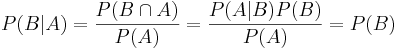 .
.
If A and B are statistically independent, then 
Multiplication Rule
For any two events (whether dependent or independent):

In general, for any collection of events:


Law of total probability
If {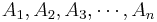 } partition the sample space S (i.e., all events are mutually exclusive and
  ) then for any event B


- Example, if A1 and A2 partition the sample space (think of males and females), then the probability of any event B (e.g., smoker) may be computed by:
P(B) = P(B | A1)P(A1) + P(B | A2)P(A2). This of course is a simple consequence of the fact that  . Therefore,
 .
.
Bayesian Rule
If {} partition the sample space S and A and B are any events (subsets of S), then:

Independence vs. disjointness/mutual-exclusiveness
- The events A and B are independent if P(A|B)=P(A). That is
- The events C and D are disjoint, or mutually-exclusive, if
 . That is
Mutual-exclusiveness and independence are different concepts. Here are two examples clarifying the differences between these concepts:
Card experiment
Suppose we play a card game of guessing the color of a randomly drawn card from a standard 52-card deck. As there are 2 possible colors (black and red), and given no other information, the chance of correctly guessing the color (e.g., black) is 0.5. However, additional information may or may not be helpful in identifying the card color. For example:
- If we know that the card denomination is a king, and there are 2 red and 2 black kings, this does not help us improve our chances of successfully identifying the correct color of the card, P(Red|King)=P(Red), independence.
- If we know that the suit of the card is heart, this does help us with correctly identifying the card color (as heart is red), P(Red|Hearts)=1.0, strong dependence as P(Red)=0.5.
- Notes:
- In both cases, the events A={Red} and B={King} and C={Hearts} are not mutually exclusive (disjoint).
- Events that are mutually exclusive (disjoint) cannot be independent.
Colorblindness experiment
Color blindness is a sex-linked trait, as many of the genes involved in color vision are on the X chromosome. Color blindness is more common in males than in females, as men do not have a second X chromosome to overwrite the chromosome which carries the mutation. If 8% of variants of a given gene are defective (mutated), the probability of a single copy being defective is 8%, but the probability that two (independent) copies are both defective is 0.08 × 0.08 = 0.0064.
- The events A={Female} and B={Color blind} are not mutually exclusive (females can be color blind), nor independent (the rate of color blindness among females is lower). Color blindness prevalence within the 2 genders is P(CB|Male) = 0.08, and P(CB|Female)=0.005, where CB={color blind, one color, a color combination, or another mutation}.
- See the Distributome Colorblindness activity.
Example
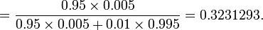
Suppose a Laboratory blood test is used as evidence for a disease. Assume P(positive Test| Disease) = 0.95, P(positive Test| no Disease)=0.01 and P(Disease) = 0.005. Find P(Disease|positive Test)=?
Denote D = {the test person has the disease}, Dc = {the test person does not have the disease} and T = {the test result is positive}. Then

See also
Problems
References
- SOCR Home page: http://www.socr.ucla.edu
Translate this page:
