SOCR EduMaterials Activities ApplicationsActivities Portfolio
From Socr
(→Portfolio Theory) |
(→Portfolio Theory) |
||
| Line 3: | Line 3: | ||
* '''Description''': You can access the portfolio applet at http://www.socr.ucla.edu/htmls/app/ . | * '''Description''': You can access the portfolio applet at http://www.socr.ucla.edu/htmls/app/ . | ||
| - | An investor has a certain amount of dollars to invest into two stocks | + | * An investor has a certain amount of dollars to invest into two stocks |
(<math>IBM</math> and <math>TEXACO</math>). A portion of the available funds will be invested into | (<math>IBM</math> and <math>TEXACO</math>). A portion of the available funds will be invested into | ||
IBM (denote this portion of the funds with <math>x_A</math>) and the remaining funds | IBM (denote this portion of the funds with <math>x_A</math>) and the remaining funds | ||
| Line 31: | Line 31: | ||
</math> | </math> | ||
<br> | <br> | ||
| - | Therefore our goal is to find <math>x_A</math> and <math>x_B</math>, the percentage of the | + | * Therefore our goal is to find <math>x_A</math> and <math>x_B</math>, the percentage of the |
available funds that will be invested in each stock. Substituting | available funds that will be invested in each stock. Substituting | ||
<math>x_B=1-x_A</math> into the equation of the variance we get | <math>x_B=1-x_A</math> into the equation of the variance we get | ||
| Line 38: | Line 38: | ||
</math> | </math> | ||
<br> | <br> | ||
| - | To minimize the above exression we take the derivative with respect to | + | * To minimize the above exression we take the derivative with respect to |
<math>x_A</math>, set it equal to zero and solve for <math>x_A</math>. The result is: | <math>x_A</math>, set it equal to zero and solve for <math>x_A</math>. The result is: | ||
<math> | <math> | ||
| Line 65: | Line 65: | ||
E(0.42R_A+0.58R_B)=0.42(0.010)+0.58(0.013)=0.01174. | E(0.42R_A+0.58R_B)=0.42(0.010)+0.58(0.013)=0.01174. | ||
</math> | </math> | ||
| - | We can try many other combinations of <math>x_A</math> and <math>x_B</math> (but always <math>x_A+x_B=1</math>) | + | * We can try many other combinations of <math>x_A</math> and <math>x_B</math> (but always <math>x_A+x_B=1</math>) |
and compute the risk and return for each resulting portfolio. This is | and compute the risk and return for each resulting portfolio. This is | ||
shown in the table and the graph below. | shown in the table and the graph below. | ||
| Line 208: | Line 208: | ||
<br> | <br> | ||
| - | For the above calculations short selling was not allowed (<math>0 \le x_A \le 1</math> and | + | * For the above calculations short selling was not allowed (<math>0 \le x_A \le 1</math> and |
<math>0 \le x_B \le 1</math>, in addition to <math>x_A+x_B=1</math>). We note here that the efficient portfolios are located on the top part of the graph between the minimum risk portfolio point and the maximum return portfolio point, which is called the efficient frontier (the blue portion of the graph). Efficient portfolios should provide higher expected return for the same level of risk or lower risk for the same level of expected return. <br> | <math>0 \le x_B \le 1</math>, in addition to <math>x_A+x_B=1</math>). We note here that the efficient portfolios are located on the top part of the graph between the minimum risk portfolio point and the maximum return portfolio point, which is called the efficient frontier (the blue portion of the graph). Efficient portfolios should provide higher expected return for the same level of risk or lower risk for the same level of expected return. <br> | ||
| - | If short sales are allowed, which means that the investor can sell a stock that he or she does not own the graph has the same shape but now with more possibilities. The investor can have very large expected return but this will be associated with very large risk. The constraint here is only <math>x_A+x_B=1</math>, since either <math>x_A<math> or <math>x_B</math> can be negative. The snapshot below from the SOCR applet shows the ``short sales scenario" for the IBM and TEXACO stocks. The blue portion of the portfolio possibilities curve occurs when short sales are allowed, while the red portion corresponds to the case when short sales are not allowed. <br> | + | * If short sales are allowed, which means that the investor can sell a stock that he or she does not own the graph has the same shape but now with more possibilities. The investor can have very large expected return but this will be associated with very large risk. The constraint here is only <math>x_A+x_B=1</math>, since either <math>x_A<math> or <math>x_B</math> can be negative. The snapshot below from the SOCR applet shows the ``short sales scenario" for the IBM and TEXACO stocks. The blue portion of the portfolio possibilities curve occurs when short sales are allowed, while the red portion corresponds to the case when short sales are not allowed. <br> |
<center>[[Image: Ibm_texaco_short_sales.jpg|600px]]</center> | <center>[[Image: Ibm_texaco_short_sales.jpg|600px]]</center> | ||
| - | When the investor faces the efficient frontier when short sales are allowed and he or she can lend or borrow at the risk-free interest rate the efficient frontier will change in the following way: Let <math>x</math> be the portion of the investor's wealth invested in portfolio <math>A</math> that lies on the efficient frontier, and <math>1-x</math> the the portion invested in a risk-free asset. This combination is a new portfolio and has | + | * When the investor faces the efficient frontier when short sales are allowed and he or she can lend or borrow at the risk-free interest rate the efficient frontier will change in the following way: Let <math>x</math> be the portion of the investor's wealth invested in portfolio <math>A</math> that lies on the efficient frontier, and <math>1-x</math> the the portion invested in a risk-free asset. This combination is a new portfolio and has |
<math> | <math> | ||
\bar R_p=x\bar R_A + (1-x)R_f | \bar R_p=x\bar R_A + (1-x)R_f | ||
| Line 232: | Line 232: | ||
<br> | <br> | ||
| - | This is an equation of a straight line. On this line we find all the possible combinations of portfolio <math>A</math> and the risk-free rate. Another investor can choose to combine the risk-free rate with portfolio <math>B</math> or portfolio <math>C</math>. Clearly, for the same level risk the combinations that lie on the <math>Rf-B</math> line have higher expected return than those on the line <math>Rf-A</math> (see figure below). And <math>Rf-C</math> will produce combinations that have higher return than those on <math>Rf-B</math> for the same level of risk, etc. <br> | + | * This is an equation of a straight line. On this line we find all the possible combinations of portfolio <math>A</math> and the risk-free rate. Another investor can choose to combine the risk-free rate with portfolio <math>B</math> or portfolio <math>C</math>. Clearly, for the same level risk the combinations that lie on the <math>Rf-B</math> line have higher expected return than those on the line <math>Rf-A</math> (see figure below). And <math>Rf-C</math> will produce combinations that have higher return than those on <math>Rf-B</math> for the same level of risk, etc. <br> |
<center>[[Image: Portfolio_risk_free_asset.jpg|600px]]</center>> | <center>[[Image: Portfolio_risk_free_asset.jpg|600px]]</center>> | ||
<br> | <br> | ||
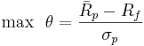
| - | The solution, therefore, is to find the point of tangency of this line to the efficient frontier. Let's call this point <math>G</math>. To find this point we want to maximize the slope of the line in (1) as follows: | + | * The solution, therefore, is to find the point of tangency of this line to the efficient frontier. Let's call this point <math>G</math>. To find this point we want to maximize the slope of the line in (1) as follows: |
<math> | <math> | ||
\mbox{max} \ \ \theta = \frac{\bar R_p - R_f}{\sigma_p} | \mbox{max} \ \ \theta = \frac{\bar R_p - R_f}{\sigma_p} | ||
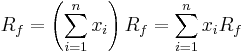
| Line 249: | Line 249: | ||
R_f=\left(\sum_{i=1}^n x_i\right) R_f = \sum_{i=1}^n x_iR_f | R_f=\left(\sum_{i=1}^n x_i\right) R_f = \sum_{i=1}^n x_iR_f | ||
</math> | </math> | ||
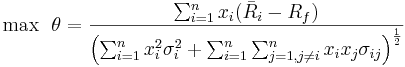
| - | + | * We can write the maximization problem as | |
<math> | <math> | ||
\mbox{max} \ \ \theta=\frac{\sum_{i=1}^n x_i (\bar R_i - R_f)} | \mbox{max} \ \ \theta=\frac{\sum_{i=1}^n x_i (\bar R_i - R_f)} | ||
| Line 262: | Line 262: | ||
</math> | </math> | ||
<br> | <br> | ||
| - | Take now the partial derivative with respect to each <math>x_i, i=1, \cdots, n</math>, set them equal to zero and solve. Let's find the partial derivative w.r.t. <math>x_k</math>: | + | * Take now the partial derivative with respect to each <math>x_i, i=1, \cdots, n</math>, set them equal to zero and solve. Let's find the partial derivative w.r.t. <math>x_k</math>: |
<math> | <math> | ||
\frac{\partial \theta}{\partial x_k} = | \frac{\partial \theta}{\partial x_k} = | ||
| Line 271: | Line 271: | ||
</math> | </math> | ||
<br> | <br> | ||
| - | Multiply both sides by | + | * Multiply both sides by |
<math> | <math> | ||
\left[\sum_{i=1}^n x_i^2 \sigma_i^2 + \sum_{i=1}^n \sum_{j=1, j \ne i}^n x_i x_j \sigma_{ij}\right]^{\frac{1}{2}} \ \ \ \mbox{to get} | \left[\sum_{i=1}^n x_i^2 \sigma_i^2 + \sum_{i=1}^n \sum_{j=1, j \ne i}^n x_i x_j \sigma_{ij}\right]^{\frac{1}{2}} \ \ \ \mbox{to get} | ||
| Line 282: | Line 282: | ||
</math> | </math> | ||
<br> | <br> | ||
| - | Now, if we let | + | * Now, if we let |
<math> | <math> | ||
\lambda= | \lambda= | ||
| Line 300: | Line 300: | ||
</math> | </math> | ||
<br> | <br> | ||
| - | Let's define now a new variable, | + | * Let's define now a new variable, |
<math> | <math> | ||
z_k = \lambda x_k | z_k = \lambda x_k | ||
| Line 310: | Line 310: | ||
\bar R_k - R_f = z_k \sigma_k^2 + \sum_{j=1, j \ne k}^n z_j \sigma_{kj} | \bar R_k - R_f = z_k \sigma_k^2 + \sum_{j=1, j \ne k}^n z_j \sigma_{kj} | ||
</math> | </math> | ||
| - | We have one equation like (2) for each <math>i=1, \cdots, n</math>. Here they are: | + | * We have one equation like (2) for each <math>i=1, \cdots, n</math>. Here they are: |
<math> | <math> | ||
\bar R_1 - R_f = z_1 \sigma_1^2 + z_2 \sigma_{12} + z_3 \sigma_{13} + \cdots + z_n \sigma_{1n} | \bar R_1 - R_f = z_1 \sigma_1^2 + z_2 \sigma_{12} + z_3 \sigma_{13} + \cdots + z_n \sigma_{1n} | ||
| Line 335: | Line 335: | ||
</math> | </math> | ||
<br> | <br> | ||
| - | The solution involves solving the system of these simultaneous equations, which can be written in matrix form as: | + | * The solution involves solving the system of these simultaneous equations, which can be written in matrix form as: |
<math> | <math> | ||
\bar R = \Sigma Z | \bar R = \Sigma Z | ||
| Line 344: | Line 344: | ||
</math> | </math> | ||
<br> | <br> | ||
| - | Once we find the <math>z_i's</math> it is easy to find the <math>x_i's</math> (the fraction of funds to be invested in each security). Earlier we defined | + | * Once we find the <math>z_i's</math> it is easy to find the <math>x_i's</math> (the fraction of funds to be invested in each security). Earlier we defined |
<math> | <math> | ||
z_k = \lambda x_k \Rightarrow x_k = \frac{z_k}{\lambda} | z_k = \lambda x_k \Rightarrow x_k = \frac{z_k}{\lambda} | ||
</math> | </math> | ||
| - | We need to find <math>\lambda</math> as follows: | + | * We need to find <math>\lambda</math> as follows: |
<math> | <math> | ||
z_1 + z_2 + \cdots + z_n = \sum_{i=1}^n z_i | z_1 + z_2 + \cdots + z_n = \sum_{i=1}^n z_i | ||
| Line 361: | Line 361: | ||
</math> | </math> | ||
<br> | <br> | ||
| - | Therefore, <br> | + | * Therefore, <br> |
<math> | <math> | ||
x_1 = \frac{z_1}{\lambda} | x_1 = \frac{z_1}{\lambda} | ||
| Line 391: | Line 391: | ||
<br> | <br> | ||
| - | The snapshot form the SOCR portfolio applet shows an example with 5 stocks. Again, the red points in the applet correspond to the case when short sales are not allowed. The point of tangency can be found with a choice of the risk-free rate that can be entered in the input dialog box. | + | * The snapshot form the SOCR portfolio applet shows an example with 5 stocks. Again, the red points in the applet correspond to the case when short sales are not allowed. The point of tangency can be found with a choice of the risk-free rate that can be entered in the input dialog box. |
<center>[[Image: Tangent_point_5_stocks.jpg|600px]]</center> | <center>[[Image: Tangent_point_5_stocks.jpg|600px]]</center> | ||
| Line 397: | Line 397: | ||
<br> | <br> | ||
| - | The materials above was partially taken from ''Modern Portfolio Theory'' by Edwin J. Elton, Martin J. Gruber, Stephen J. Brown, and William N. Goetzmann, Sixth Edition, Wiley, 2003. | + | * The materials above was partially taken from ''Modern Portfolio Theory'' by Edwin J. Elton, Martin J. Gruber, Stephen J. Brown, and William N. Goetzmann, Sixth Edition, Wiley, 2003. |
Revision as of 15:28, 3 August 2008
Portfolio Theory
- Description: You can access the portfolio applet at http://www.socr.ucla.edu/htmls/app/ .
- An investor has a certain amount of dollars to invest into two stocks
(IBM and TEXACO). A portion of the available funds will be invested into
IBM (denote this portion of the funds with xA) and the remaining funds
into TEXACO (denote it with xB) - so xA + xB = 1. The resulting portfolio
will be xARA + xBRB, where RA is the monthly return of IBM and RB is the
monthly return of TEXACO. The goal here is to
find the most efficient portfolios given a certain amount of risk.
Using market data from January 1980 until February 2001 we compute
that E(RA) = 0.010, E(RB) = 0.013, Var(RA) = 0.0061, Var(RB) = 0.0046, and
Cov(RA,RB) = 0.00062. We first want to minimize the variance of the portfolio.
This will be:

 Or
Or

- Therefore our goal is to find xA and xB, the percentage of the
available funds that will be invested in each stock. Substituting
xB = 1 − xA into the equation of the variance we get

- To minimize the above exression we take the derivative with respect to
xA, set it equal to zero and solve for xA. The result is:
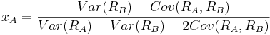
and therefore
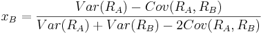
The values of xA and xB are:
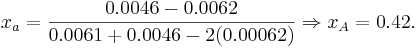 and
and  . Therefore if the investor invests
 of the available funds into IBM and the remaining
  into TEXACO the variance of the portfolio will be minimum and equal to:
Var(0.42RA + 0.58RB) = 0.422(0.0061) + 0.582(0.0046) + 2(0.42)(0.58)(0.00062) = 0.002926.
The corresponding expected return of this porfolio will be:
E(0.42RA + 0.58RB) = 0.42(0.010) + 0.58(0.013) = 0.01174.
into TEXACO the variance of the portfolio will be minimum and equal to:
Var(0.42RA + 0.58RB) = 0.422(0.0061) + 0.582(0.0046) + 2(0.42)(0.58)(0.00062) = 0.002926.
The corresponding expected return of this porfolio will be:
E(0.42RA + 0.58RB) = 0.42(0.010) + 0.58(0.013) = 0.01174.
- We can try many other combinations of xA and xB (but always xA + xB = 1)
and compute the risk and return for each resulting portfolio. This is shown in the table and the graph below.
| xA | xB | Risk (σ2) | Return | Risk (σ) |
|---|---|---|---|---|
| 1.00 | 0.00 | 0.006100 | 0.01000 | 0.078102 |
| 0.95 | 0.05 | 0.005576 | 0.01015 | 0.074670 |
| 0.90 | 0.10 | 0.005099 | 0.01030 | 0.071404 |
| 0.85 | 0.15 | 0.004669 | 0.01045 | 0.068329 |
| 0.80 | 0.20 | 0.004286 | 0.01060 | 0.065471 |
| 0.75 | 0.25 | 0.003951 | 0.01075 | 0.062859 |
| 0.70 | 0.30 | 0.003663 | 0.01090 | 0.060526 |
| 0.65 | 0.35 | 0.003423 | 0.01105 | 0.058505 |
| 0.60 | 0.40 | 0.003230 | 0.01120 | 0.056830 |
| 0.55 | 0.45 | 0.003084 | 0.01135 | 0.055531 |
| 0.50 | 0.50 | 0.002985 | 0.01150 | 0.054635 |
| 0.42 | 0.58 | 0.002926 | 0.01174 | 0.054088 |
| 0.40 | 0.60 | 0.002930 | 0.01180 | 0.054126 |
| 0.35 | 0.65 | 0.002973 | 0.01195 | 0.054524 |
| 0.30 | 0.70 | 0.003063 | 0.01210 | 0.055348 |
| 0.25 | 0.75 | 0.003201 | 0.01225 | 0.056580 |
| 0.20 | 0.80 | 0.003386 | 0.01240 | 0.058193 |
| 0.15 | 0.85 | 0.003619 | 0.01255 | 0.060157 |
| 0.10 | 0.90 | 0.003899 | 0.01270 | 0.062439 |
| 0.05 | 0.95 | 0.004226 | 0.01285 | 0.065005 |
| 0.00 | 1.00 | 0.004600 | 0.01300 | 0.067823 |

- For the above calculations short selling was not allowed (
 and
and
 , in addition to xA + xB = 1). We note here that the efficient portfolios are located on the top part of the graph between the minimum risk portfolio point and the maximum return portfolio point, which is called the efficient frontier (the blue portion of the graph). Efficient portfolios should provide higher expected return for the same level of risk or lower risk for the same level of expected return.
- If short sales are allowed, which means that the investor can sell a stock that he or she does not own the graph has the same shape but now with more possibilities. The investor can have very large expected return but this will be associated with very large risk. The constraint here is only xA + xB = 1, since either xA < math > or < math > xB can be negative. The snapshot below from the SOCR applet shows the ``short sales scenario" for the IBM and TEXACO stocks. The blue portion of the portfolio possibilities curve occurs when short sales are allowed, while the red portion corresponds to the case when short sales are not allowed.

- When the investor faces the efficient frontier when short sales are allowed and he or she can lend or borrow at the risk-free interest rate the efficient frontier will change in the following way: Let x be the portion of the investor's wealth invested in portfolio A that lies on the efficient frontier, and 1 − x the the portion invested in a risk-free asset. This combination is a new portfolio and has
where Rf is the return of the risk-free asset. The variance of this combination is simply
From the last two equations we get
- This is an equation of a straight line. On this line we find all the possible combinations of portfolio A and the risk-free rate. Another investor can choose to combine the risk-free rate with portfolio B or portfolio C. Clearly, for the same level risk the combinations that lie on the Rf − B line have higher expected return than those on the line Rf − A (see figure below). And Rf − C will produce combinations that have higher return than those on Rf − B for the same level of risk, etc.

- The solution, therefore, is to find the point of tangency of this line to the efficient frontier. Let's call this point G. To find this point we want to maximize the slope of the line in (1) as follows:
 Subject to
 Since,
- We can write the maximization problem as
or
![\mbox{max} \ \ \theta=\left[\sum_{i=1}^n x_i (\bar R_i - R_f)\right]
\left[\sum_{i=1}^n x_i^2 \sigma_i^2 + \sum_{i=1}^n \sum_{j=1, j \ne i}^n x_i x_j \sigma_{ij}\right]^{-\frac{1}{2}}](/socr/uploads/math/0/b/9/0b9de3e6da1231d579ef5f43fc8f1853.png)
- Take now the partial derivative with respect to each
 , set them equal to zero and solve. Let's find the partial derivative w.r.t. xk:
![\frac{\partial \theta}{\partial x_k} =
(\bar R_k - R_f)\left[\sum_{i=1}^n x_i^2 \sigma_i^2 + \sum_{i=1}^n \sum_{j=1, j \ne i}^n x_i x_j \sigma_{ij}\right]^{-\frac{1}{2}} +
\left[\sum_{i=1}^n x_i(\bar R_i - R_f)\right]
\left[2x_k\sigma_k^2 + 2 \sum_{j=1, j \ne k}^n x_j \sigma_{kj}\right] \times
\left[\sum_{i=1}^n x_i^2 \sigma_i^2 + \sum_{i=1}^n \sum_{j=1, j \ne i}^n x_i x_j \sigma_{ij}\right]^{-\frac{3}{2}} \times (-\frac{1}{2}) = 0](/socr/uploads/math/3/b/2/3b21c3cbb8fe3b48c09781505085fe88.png)
- Multiply both sides by
![\left[\sum_{i=1}^n x_i^2 \sigma_i^2 + \sum_{i=1}^n \sum_{j=1, j \ne i}^n x_i x_j \sigma_{ij}\right]^{\frac{1}{2}} \ \ \ \mbox{to get}](/socr/uploads/math/d/7/2/d728e973c6bb13199932fffe13b06f76.png)

- Now, if we let
the previous expression will be
or
- Let's define now a new variable,
zk = λxk
and finally
- We have one equation like (2) for each
 . Here they are:


- The solution involves solving the system of these simultaneous equations, which can be written in matrix form as:
 where Σ is the variance-covariance matrix of the returns of the n stocks. To solve for Z:

- Once we find the zi's it is easy to find the xi's (the fraction of funds to be invested in each security). Earlier we defined
- We need to find λ as follows:
- Therefore,


- The snapshot form the SOCR portfolio applet shows an example with 5 stocks. Again, the red points in the applet correspond to the case when short sales are not allowed. The point of tangency can be found with a choice of the risk-free rate that can be entered in the input dialog box.

- The materials above was partially taken from Modern Portfolio Theory by Edwin J. Elton, Martin J. Gruber, Stephen J. Brown, and William N. Goetzmann, Sixth Edition, Wiley, 2003.
