SOCR EduMaterials Activities ExpCarTimeExperiment
From Socr
m |
m |
||
| (9 intermediate revisions not shown) | |||
| Line 3: | Line 3: | ||
== Description == | == Description == | ||
| - | + | This activity presents details about Exponential, Poisson and Gamma processes, simulations, estimation and model-fitting. It also provides a specific framework for hands-on demonstration of all these concepts using [http://socr.ucla.edu/htmls/SOCR_Experiments.html SOCR Java applets] via an experiment simulating between-card times of cars driving on a freeway. | |
| - | + | ||
== Goal == | == Goal == | ||
To provide an interactive simulation demonstrating exponential processes, exponential decay, simulation and model fitting. Additional aims are to: | To provide an interactive simulation demonstrating exponential processes, exponential decay, simulation and model fitting. Additional aims are to: | ||
| - | * Draw | + | * Draw analogies between [http://en.wikipedia.org/wiki/Gamma_distribution Gamma], [http://en.wikipedia.org/wiki/Exponential_distribution Exponential] and [http://en.wikipedia.org/wiki/Poisson_distribution Poisson] (discrete!) |
* Provide the means for (large) data generation/sampling | * Provide the means for (large) data generation/sampling | ||
* Provide the infrastructure for model-fitting and assessment. | * Provide the infrastructure for model-fitting and assessment. | ||
| Line 21: | Line 20: | ||
Select the '''number of cars (k)''' and the '''rate of the exponential process (r)'''. When pressing the '''play''' button, one trial will be executed that involves sampling k random exponential time variables (representing the between car times). The results will be displayed graphically in the two graph windows (timeline and histogram) for this process. Summary statistics and model vs. data distributions are shown in the distribution table below. The '''stop''' button ceases any activity and is helpful when the experimenter chooses a large number of cars (k is large). The '''reset''' button will clear and re-initialize the entire experiment, deleting all previous information and data collected. | Select the '''number of cars (k)''' and the '''rate of the exponential process (r)'''. When pressing the '''play''' button, one trial will be executed that involves sampling k random exponential time variables (representing the between car times). The results will be displayed graphically in the two graph windows (timeline and histogram) for this process. Summary statistics and model vs. data distributions are shown in the distribution table below. The '''stop''' button ceases any activity and is helpful when the experimenter chooses a large number of cars (k is large). The '''reset''' button will clear and re-initialize the entire experiment, deleting all previous information and data collected. | ||
| + | In this experiment, '''cars''' are represented as square-dots of different colors on the top graph. The distance between the car position and the origin illustrates the distance between this car and the one ahead of it. The further to the right a car is on this timeline graph, the further from its preceding car (further back in time) it is. | ||
| + | |||
| + | |||
As the number of cars (k) increases, the distribution of the between-car times will have exponential-decay shape. Note that as the number of cars (k) increases, the empirical histogram (graph) and moments (table) of the random exponential times begin to converge to their corresponding Exponential distribution counterparts. Arrows point to the match of the empirical histogram of the between-car times and theoretical Exponential distribution, the random sample of between-car times (Y column of left table) and the similarity between the first two moments of the sample data and model (Exponential) distributions. | As the number of cars (k) increases, the distribution of the between-car times will have exponential-decay shape. Note that as the number of cars (k) increases, the empirical histogram (graph) and moments (table) of the random exponential times begin to converge to their corresponding Exponential distribution counterparts. Arrows point to the match of the empirical histogram of the between-car times and theoretical Exponential distribution, the random sample of between-car times (Y column of left table) and the similarity between the first two moments of the sample data and model (Exponential) distributions. | ||
| Line 27: | Line 29: | ||
== Applications == | == Applications == | ||
| - | === | + | ===Relations between [http://en.wikipedia.org/wiki/Gamma_distribution Gamma], [http://en.wikipedia.org/wiki/Exponential_distribution Exponential] and [http://en.wikipedia.org/wiki/Poisson_distribution Poisson] distributions=== |
Number of Arrivals in a fixed time-period follows Poisson distribution. | Number of Arrivals in a fixed time-period follows Poisson distribution. | ||
| + | * <math>{\Gamma}(k=1, \theta=1/\lambda)\,</math> reduces to an Exponential distribution with rate parameter <math>\lambda</math>. | ||
| + | * For an integer <math>k</math> parameter, the Gamma distribution <math>{\Gamma}(k=1, \theta=1/\lambda)\,</math> becomes the probability distribution of the waiting time until the <math>k^{th}</math> ''arrival'' of a one-dimensional Poisson process with expected number of arrivals in a fixed time interval equal to <math>\lambda = {1\over \theta}</math>. | ||
| + | * If one observes a Poisson process (number of arrivals in a fixed time-interval), then the Exponential distribution describes the lengths of the inter-arrival times in the homogeneous Poisson processes. | ||
| + | * The Exponential distribution may also be considered as a continuous analog of the [http://en.wikipedia.org/wiki/Geometric_distribution Geometric distribution]. Geometric distribution describes the number of Bernoulli trials until the first change (success). Similarly, Exponential distribution describes the time for a continuous process to change state and is sometimes called the '''Mean-Time-to-Failure''' distribution. | ||
| + | |||
=== Exponential data sampling=== | === Exponential data sampling=== | ||
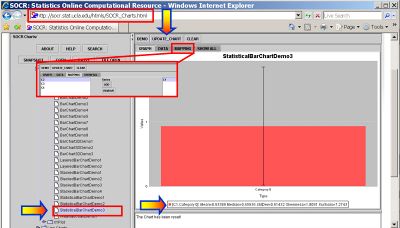
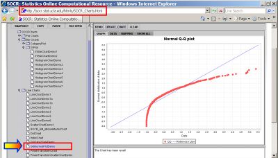
| - | We can use this applet to | + | We can use this applet to generate a sample of an arbitrary size from an Exponential Distribution with specified rate parameter. Then these data may be used for simulations or exploratory data analysis. For example, suppose we ran the experiment with k=1,000, as shown on the image above. We can copy the sample from the '''Y''' column and past it in any of the [http://socr.ucla.edu/htmls/SOCR_Charts.html SOCR Charts]. The image below shows the construction of a ''Statistical Bar Chart'' using the 1,000 Exponential (between-car) time measurements. Notice how the summary statistics on this Bar Chart coincide with the data-statistics reported on the distribution table of the Exponential Time Car Experiment applet. The last graph (bottom-right) illustrates a (Q-Q) plot of the Normal vs. Exponential-sample quantiles. The highly non-linear shape of this QQ plot indicates the significant departure of normality of these Exponential time measurements (between-car times). |
<center>[[Image:SOCR_Activities_ExpCarTimeExperiment_Dinov_011908_Fig3.jpg|400px]] | <center>[[Image:SOCR_Activities_ExpCarTimeExperiment_Dinov_011908_Fig3.jpg|400px]] | ||
| - | [[Image: | + | [[Image:SOCR_Activities_ExpCarTimeExperiment_Dinov_011908_Fig5.jpg|400px]]</center> |
| - | <center>[[Image:SOCR_Activities_ExpCarTimeExperiment_Dinov_011908_Fig6.jpg|400px]]</center> | + | <center>[[Image:SOCR_Activities_ExpCarTimeExperiment_Dinov_011908_Fig6.jpg|400px]] |
| + | [[Image:SOCR_Activities_ExpCarTimeExperiment_Dinov_011908_Fig7.jpg|400px]]</center> | ||
===Exponential model-fitting and assessment=== | ===Exponential model-fitting and assessment=== | ||
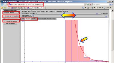
| + | The image below demonstrates how we can fit a Gamma-model to the sample of (k=1,000) Exponential measurements that we simulated as between-car times. Go to [http://socr.ucla.edu/htmls/SOCR_Modeler.html SOCR Modeler] and click the ''Raw Data'' check-box. Then paste in all of your raw Exponential measurements recorder in the '''Y''' column of the '''Exponential Time Car Experiment'''. Choose '''Gamma-Fit''', from the drop-down list of SOCR modelers on the top-left. Click on the ''Estimate parameters'' and ''Scale up'' check-boxes. Then go to the Graph tab and use the sliders on the top to select an appropriate view for the data and the model-fit. Under the Results tab you will find the Gamma model parameter estimates (these are [http://en.wikipedia.org/wiki/Maximum_likelihood_estimate MLE estimates]). In this case, the best Gamma distribution model is estimated to have parameters ''Shape = 0.8942640916359458; Scale = 1.0443144529333228''. Note the similarities between these estimates and what we expect, according to our simulation above, <math>Exp(\lambda=1.02)=Gamma(1, 1/1.02)</math>. | ||
| + | |||
| + | <center>[[Image:SOCR_Activities_ExpCarTimeExperiment_Dinov_011908_Fig8.jpg|400px]]</center> | ||
{{translate|pageName=http://wiki.stat.ucla.edu/socr/index.php?title=SOCR_EduMaterials_Activities_ExpCarTimeExperiment}} | {{translate|pageName=http://wiki.stat.ucla.edu/socr/index.php?title=SOCR_EduMaterials_Activities_ExpCarTimeExperiment}} | ||
Current revision as of 01:57, 21 January 2008
Contents |
Exponential Time Car Activity
Description
This activity presents details about Exponential, Poisson and Gamma processes, simulations, estimation and model-fitting. It also provides a specific framework for hands-on demonstration of all these concepts using SOCR Java applets via an experiment simulating between-card times of cars driving on a freeway.
Goal
To provide an interactive simulation demonstrating exponential processes, exponential decay, simulation and model fitting. Additional aims are to:
- Draw analogies between Gamma, Exponential and Poisson (discrete!)
- Provide the means for (large) data generation/sampling
- Provide the infrastructure for model-fitting and assessment.
Experiment
Go to the SOCR Experiments and select the Exponential Car-Time Experiment from the drop-down list of experiments on the top left. The image below shows the initial view of this experiment with pointers and highlights of the most important components and controls:
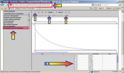
Select the number of cars (k) and the rate of the exponential process (r). When pressing the play button, one trial will be executed that involves sampling k random exponential time variables (representing the between car times). The results will be displayed graphically in the two graph windows (timeline and histogram) for this process. Summary statistics and model vs. data distributions are shown in the distribution table below. The stop button ceases any activity and is helpful when the experimenter chooses a large number of cars (k is large). The reset button will clear and re-initialize the entire experiment, deleting all previous information and data collected.
In this experiment, cars are represented as square-dots of different colors on the top graph. The distance between the car position and the origin illustrates the distance between this car and the one ahead of it. The further to the right a car is on this timeline graph, the further from its preceding car (further back in time) it is.
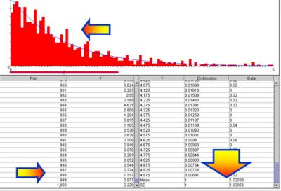
As the number of cars (k) increases, the distribution of the between-car times will have exponential-decay shape. Note that as the number of cars (k) increases, the empirical histogram (graph) and moments (table) of the random exponential times begin to converge to their corresponding Exponential distribution counterparts. Arrows point to the match of the empirical histogram of the between-car times and theoretical Exponential distribution, the random sample of between-car times (Y column of left table) and the similarity between the first two moments of the sample data and model (Exponential) distributions.
Applications
Relations between Gamma, Exponential and Poisson distributions
Number of Arrivals in a fixed time-period follows Poisson distribution.
-
 reduces to an Exponential distribution with rate parameter λ.
- For an integer k parameter, the Gamma distribution
 becomes the probability distribution of the waiting time until the kth arrival of a one-dimensional Poisson process with expected number of arrivals in a fixed time interval equal to
  .
.
- If one observes a Poisson process (number of arrivals in a fixed time-interval), then the Exponential distribution describes the lengths of the inter-arrival times in the homogeneous Poisson processes.
- The Exponential distribution may also be considered as a continuous analog of the Geometric distribution. Geometric distribution describes the number of Bernoulli trials until the first change (success). Similarly, Exponential distribution describes the time for a continuous process to change state and is sometimes called the Mean-Time-to-Failure distribution.
Exponential data sampling
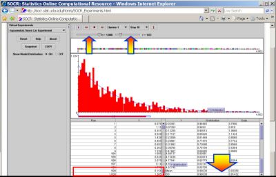
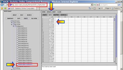
We can use this applet to generate a sample of an arbitrary size from an Exponential Distribution with specified rate parameter. Then these data may be used for simulations or exploratory data analysis. For example, suppose we ran the experiment with k=1,000, as shown on the image above. We can copy the sample from the Y column and past it in any of the SOCR Charts. The image below shows the construction of a Statistical Bar Chart using the 1,000 Exponential (between-car) time measurements. Notice how the summary statistics on this Bar Chart coincide with the data-statistics reported on the distribution table of the Exponential Time Car Experiment applet. The last graph (bottom-right) illustrates a (Q-Q) plot of the Normal vs. Exponential-sample quantiles. The highly non-linear shape of this QQ plot indicates the significant departure of normality of these Exponential time measurements (between-car times).
Exponential model-fitting and assessment
The image below demonstrates how we can fit a Gamma-model to the sample of (k=1,000) Exponential measurements that we simulated as between-car times. Go to SOCR Modeler and click the Raw Data check-box. Then paste in all of your raw Exponential measurements recorder in the Y column of the Exponential Time Car Experiment. Choose Gamma-Fit, from the drop-down list of SOCR modelers on the top-left. Click on the Estimate parameters and Scale up check-boxes. Then go to the Graph tab and use the sliders on the top to select an appropriate view for the data and the model-fit. Under the Results tab you will find the Gamma model parameter estimates (these are MLE estimates). In this case, the best Gamma distribution model is estimated to have parameters Shape = 0.8942640916359458; Scale = 1.0443144529333228. Note the similarities between these estimates and what we expect, according to our simulation above, Exp(λ = 1.02) = Gamma(1,1 / 1.02).
Translate this page:
