SOCR EduMaterials Activities GeneralCentralLimitTheorem

From Socr

Revision as of 21:46, 22 January 2007

SOCR Educational Materials - Activities - SOCR General Central Limit Theorem (CLT) Activity

This activity represents a very general demonstration of the effects of the Central Limit Theorem (CLT). The activity is based on the SOCR Sampling Distribution CLT Experiment. This experiment builds upon a RVLS CLT applet by extending the applet functionality and providing the capability of sampling from any SOCR Distribution.

• Goals: The aims of this activity are to
  • provide intuitive notion of sampling from any process with a well-defined distribution
  • motivate and facilitate learning of the central limit theorem
  • emperically validate that sample-averages of random observations (most processes) follow approximately normal distribution
  • emperacally demonstrate that the sample-average is special and other sample statistics (e.g., median, variance, range, etc.) generally do not have distributions that are normal
  • illustrate that the expectation of the sample-average equals the population mean (and the sample-average is typically a good measure of centrality for a population/process)
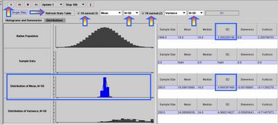
  • show that the variation of the sample average rapidly decreases as the sample size increases ().

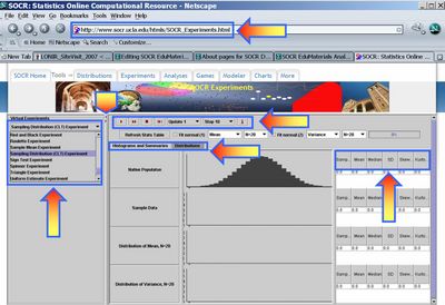
• The SOCR CLT Experiment: To start the this Experiment, go to SOCR Experiments and select the SOCR Sampling Distribution CLT Experiment from the drop-down list of experiments in the left panel. The image below shows the interface to this experiment. Notice the main control widgets on this image (boxed in blue and pointed to by arrows). The generic control buttons on the top allow you to one or multiple steps/runs, stop and reset this experiment. The two tabs in the main frame provide graphical access the to results of the experiment (Histograms and Sumamries) or the Distribution selection panel (Distributions).

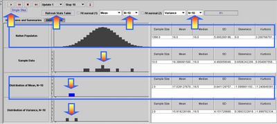
• Experiment 1: Expand your Experiment panel (right panel). Choose the two sample sizes for the two statistics to be 10. Press the step button a few of times (2-5) to see the experiment run several times. Notice how data is being sampled from the native population (the distribution of the process on the top). For each step, the process of sampling 2 samples of 10 observations will generate 2 sample statistics of the 2 population parameters of interest (these are defaulted to mean and variance). At each step, you can see the plots of all sample values, as well as the computed sample statistics for each parameter. The sample values are shown on the second row graph, below the distribution of the process, and the two sample statistics are plotted on the bottom two rows. If we run this experiment many times, the bottom two graphs become the histograms of the corresponding sample statistics. If we did this infinitely many times these two graphs become the sampling distributions of the chosen sample statistics (as the observations/measurements are independent within each sample and between samples). Finally, press the Refresh Stats Table button on the top to see the sample summary statistics for the native population distribution (row 1), last sample (row 2) and the two sample parameter estimates, mean and variance, in this case (rows 3 and 4).

• Experiment 2:

• SOCR Home page: http://www.socr.ucla.edu

Translate this page: