SOCR EduMaterials Activities General CI Experiment
From Socr
SOCR Experiments Activities - General Confidence Interval Activity
Summary
There are two types of parameter estimates – point-based and interval-based estimates. Point-estimates refer to unique quantitative estimates of various parameters. Interval-estimates represent ranges of plausible values for the parameters of interest. There are different algorithmic approaches, prior assumptions and principals for computing data-driven parameter estimates. Both point and interval estimates depend on the distribution of the process of interest, the available computational resources and other criteria that may be desirable (Stewarty 1999) – e.g., biasness and robustness of the estimates. Accurate, robust and efficient parameter estimation is critical in making inference about observable experiments, summarizing process characteristics and prediction of experimental behaviors.
This activity demonstrates the usage and functionality of SOCR General Confidence Interval Applet. This applet is complementary to the SOCR Simple Confidence Interval Applet and its corresponding activity.
Goals
The aims of this activity is to:
- TBD
- TBD
- TBD.
Motivational example

A 2005 study proposing a new computational brain atlas for Alzheimer’s disease (Mega et al., 2005) investigated the mean volumetric characteristics and the spectra of shapes and sizes of different cortical and subcortical brain regions for Alzheimer’s patients, individuals with minor cognitive impairment and asymptomatic subjects. This study estimated a number of centrality and variability parameters for these thee populations. Based on these point- and interval-estimates, the study analyzed a number of digital scans to derive criteria for imaging-based classification of subjects based on the intensities of their 3D brain scans. Their results enabled a number of subsequent inference studies that quantified the effects of subject demographics (e.g., education level, familial history, APOE allele, etc.), stage of the disease and the efficacy of new drug treatments targeting Alzheimer’s disease. The Figure to the right illustrates the shape, center and distribution parameters for the 3D geometric structure of the right hippocampus in the Alzheimer’s disease brain atlas. New imaging data can then be coregistered and compared relative to the amount of anatomical variability encoded in this atlas. This enables automated, efficient and quantitative inference on large number of brain volumes. Examples of point and interval estimates computed in this atlas framework include the mean-intensity and mean shape location, and the standard deviation of intensities and the mean deviation of shape, respectively.
Activity
Confidence intervals (CI) for the population mean μ of normal population with known population variance σ2
Let 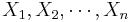 be a random sample from N(μ,σ). We know that
 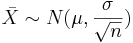 . Therefore,
-
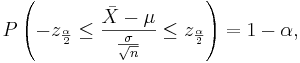
- where
 and
and  are defined as shown in the figure below:

The area 1 − α is called confidence level. Usually, the choices for confidence levels are the following:
| 1 − α |
|
|---|---|
| 0.90 | 1.645 |
| 0.95 | 1.960 |
| 0.98 | 2.325 |
| 0.99 | &2.575 |
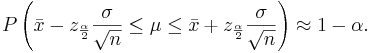
The expression above can be written as:
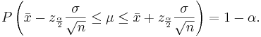
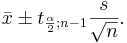
We say that we are 1 − α confident that the mean μ falls in the interval  .
.
Example 1
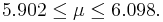
Suppose that the length of iron rods from a certain factory follows the normal distribution with known standard deviation  but unknown mean μ. Construct a 95% confidence interval for the population mean μ if a random sample of n=16 of these iron rods has sample mean
  .
.
- We solve this problem by using our CI recipe
-
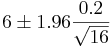
-

-
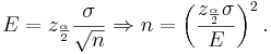
Sample size determination for a given length of the confidence interval
Find the sample size n needed when we want the width of the confidence interval to be  with confidence level 1 − α.
Solution
In the expression the width of the confidence interval is given by  (also called margin of error). We want this width to be equal to E. Therefore,
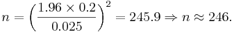
Example 2
Following our first example above, suppose that we want the entire width of the confidence interval to be equal to  . Find the sample size n needed.
Introduction of the SOCR Confidence Interval Applet
To access the SOCR applet on confidence intervals go to http://socr.ucla.edu/htmls/exp/Confidence_Interval_Experiment_General.html. To select the type and parameters of the specific confidence interval of interest click on the Confidence Interval button on the top -- this will open a new pop-up window as shown below:


A confidence interval of interest can be selected from the drop-down list under CI Settings. In this case, we selected Mean - Population Variance Known.

In the same pop-up window, under SOCR Distributions, the drop-down menu offers a list of all the available distributions of SOCR. These distributions are the same as the ones included in the SOCR Distributions applet.

Once the desired distribution is selected, its parameters can be chosen numerically or via the sliders. In this example we select:
- normal distribution with mean 5 and standard deviation 2,
- sample size (number of observations selected from the distribution) is 20,
- the confidence level (1-alpha=0.95), and
- the number of intervals to be constructed is 50 (see screenshot below).
- Note: Make sure to hit enter after you enter any of the parameters above.

To run the SOCR CI simulation, go back to the applet in the main browser window. We can run the experiment once, by clicking on the Step button, or many times by clicking on the Run button. The number of experiments can be controlled by the value of the Number of Experiments variable (10, 100, 1,000, 10,000, or continuously).

In the screenshot above we observe the following:
- The shape of the distribution that was selected (in this case Normal).
- The observations selected from the distribution for the construction of each of the 50 intervals shown in blue on the top-left graph panel.
- The confidence intervals shown as red line segments on the bottom-left panel.
- The green dots represent instances of confidence intervals that do not include the estimated parameter (in this case population mean of 5).
- All the parameters and simulation results are summarized on the right panel of the applet.
Practice
Run the same experiment using sample sizes of 20, 30, 40, 50 with the same confidence level (1 − alpha = 0.95). What are your observations and conclusions?
Confidence intervals for the population mean μ with known population variance σ2
From the central limit theorem we know that when the sample size is large (usually  ) the distribution of the sample mean
  approximately follows
 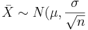 . Therefore, the confidence interval for the population mean μ is approximately given by the expression we previously discussed:
The mean μ falls in the interval .
Also, the sample size determination is given by the same formula:
Example 3
A sample of size n=50 is taken from the production of light bulbs at a certain factory. The sample mean of the lifetime of these 50 light bulbs is found to be  hours. Assume
that the population standard deviation is σ = 120 hours.
hours. Assume
that the population standard deviation is σ = 120 hours.
- Construct a 95% confidence interval for μ.
- Construct a 99% confidence interval for μ.
- What sample size is needed so that the length of the interval is 30 hours with 95% confidence?
An empirical investigation
Two dice are rolled and the sum X of the two numbers that occurred is recorded. The probability distribution of X is as follows:
| X | 2 | 3 | 4 | 5 | 6 | 7 | 8 | 9 | 10 | 11 | 12 |
|---|---|---|---|---|---|---|---|---|---|---|---|
| P(X) | 1/36 | 2/36 | 3/36 | 4/36 | 5/36 | 6/36 | 5/36 | 4/36 | 3/36 | 2/36 | 1/36 |
This distribution has mean μ = 7 and standard deviation σ = 2.42. We take 100 samples of size n=50 each from this distribution and compute for each sample the sample mean  . Pretend now that we only know that σ = 2.42, and that μ is unknown. We are going to use these 100 sample means to construct 100 confidence intervals. each one with 95% confidence level for the true population mean μ. Here are the results:
| Sample | | 95% CI for μ: 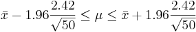 | Is μ = 7 included? |
|---|---|---|---|
| 1 | 6.9 | 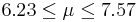 | YES |
| 2 | 6.3 |  | NO |
| 3 | 6.58 |  | YES |
| 4 | 6.54 |  | YES |
| 5 | 6.7 |  | YES |
| 6 | 6.58 | | YES |
| 7 | 7.2 |  | YES |
| 8 | 7.62 |  | YES |
| 9 | 6.94 |  | YES |
| 10 | 7.36 |  | YES |
| 11 | 7.06 |  | YES |
| 12 | 7.08 |  | YES |
| 13 | 7.42 |  | YES |
| 14 | 7.42 | | YES |
| 15 | 6.8 |  | YES |
| 16 | 6.94 | | YES |
| 17 | 7.2 | | YES |
| 18 | 6.7 | | YES |
| 19 | 7.1 |  | YES |
| 20 | 7.04 |  | YES |
| 21 | 6.98 |  | YES |
| 22 | 7.18 |  | YES |
| 23 | 6.8 | | YES |
| 24 | 6.94 | | YES |
| 25 | 8.1 |  | NO |
| 26 | 7 |  | YES |
| 27 | 7.06 | | YES |
| 28 | 6.82 |  | YES |
| 29 | 6.96 |  | YES |
| 30 | 7.46 |  | YES |
| 31 | 7.04 | | YES |
| 32 | 7.06 | | YES |
| 33 | 7.06 | | YES |
| 34 | 6.8 | | YES |
| 35 | 7.12 |  | YES |
| 36 | 7.18 | | YES |
| 37 | 7.08 | | YES |
| 38 | 7.24 |  | YES |
| 39 | 6.82 | | YES |
| 40 | 7.26 |  | YES |
| 41 | 7.34 |  | YES |
| 42 | 6.62 |  | YES |
| 43 | 7.1 | | YES |
| 44 | 6.98 | | YES |
| 45 | 6.98 | | YES |
| 46 | 7.06 | | YES |
| 47 | 7.14 |  | YES |
| 48 | 7.5 |  | YES |
| 49 | 7.08 | | YES |
| 50 | 7.32 |  | YES |
| 51 | 6.54 | | YES |
| 52 | 7.14 | | YES |
| 53 | 6.64 |  | YES |
| 54 | 7.46 | | YES |
| 55 | 7.34 | | YES |
| 56 | 7.28 |  | YES |
| 57 | 6.56 |  | YES |
| 58 | 7.72 |  | NO |
| 59 | 6.66 |  | YES |
| 60 | 6.8 | | YES |
| 61 | 7.08 | | YES |
| 62 | 6.58 | | YES |
| 63 | 7.3 |  | YES |
| 64 | 7.1 | | YES |
| 65 | 6.68 |  | YES |
| 66 | 6.98 | | YES |
| 67 | 6.94 | | YES |
| 68 | 6.78 |  | YES |
| 69 | 7.2 | | YES |
| 70 | 6.9 | | YES |
| 71 | 6.42 |  | YES |
| 72 | 6.48 |  | YES |
| 73 | 7.12 | | YES |
| 74 | 6.9 | | YES |
| 75 | 7.24 | | YES |
| 76 | 6.6 |  | YES |
| 77 | 7.28 | | YES |
| 78 | 7.18 | | YES |
| 79 | 6.76 |  | YES |
| 80 | 7.06 | | YES |
| 81 | 7 | | YES |
| 82 | 7.08 | | YES |
| 83 | 7.18 | | YES |
| 84 | 7.26 | | YES |
| 85 | 6.88 |  | YES |
| 86 | 6.28 |  | NO |
| 87 | 7.06 | | YES |
| 88 | 6.66 | | YES |
| 89 | 7.18 | | YES |
| 90 | 6.86 |  | YES |
| 91 | 6.96 | | YES |
| 92 | 7.26 | | YES |
| 93 | 6.68 | | YES |
| 94 | 6.76 | | YES |
| 95 | 7.3 | | YES |
| 96 | 7.04 | | YES |
| 97 | 7.34 | | YES |
| 98 | 6.72 |  | YES |
| 99 | 6.64 | | YES |
| 100 | 7.3 | | YES |
We observe that four confidence intervals among the 100 that we constructed fail to include the true population mean μ = 7 (about 5%).
Example 4
For this example, we will select the Exponential distribution with λ = 5 (mean of 1/5 = 0.2), sample size 60, confidence level 0.95, and number of intervals 50. These settings, along with the results of the simulations are shown below


Confidence intervals for the population mean of normal distribution when the population variance σ2 is unknown
Let be a random sample from N(μ,σ2). It is known that 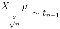 . Therefore,
-
- where
 and
and  are defined as follows:

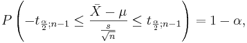
As before, the area 1 − α is called confidence level. The values of can be found from:
- SOCR Studnet's T-distribution, interactive applet, or
- SOCR T-table, below are some examples:
| 1 − α | n |
|
|---|---|---|
| 0.90 | 13 | 1.782 |
| 0.95 | 21 | 2.086 |
| 0.98 | 31 | 2.457e |
| 0.99 | 61 | 2.660 |
- Note: The sample standard deviation is computed as follows:
-
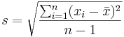
- or using the shortcut formula.
![s=\sqrt{\frac{1}{n-1}\left[\sum_{i=1}^{n} x_i^2 -
\frac{(\sum_{i=1}^{n} x_i)^2}{n}\right]}](/socr/uploads/math/f/7/a/f7a9fd62f318ce7686723617d75ead36.png)
After some rearranging the expression above can be written as:
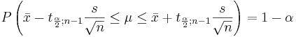
We say that we are 1 − α confident that μ falls in the interval:
Example 3
The daily production of a chemical product last week in tons was: 785, 805, 790, 793, and 802.
- Construct a 95% confidence interval for the population mean μ.
- What assumptions are necessary?
SOCR investigation
For this case, we will select the normal distribution with mean 5 and standard deviation 2, sample size of 25, number of intervals 50, and confidence level 0.95. These settings and simulation results are shown below:


We observe that the length of the confidence interval differs for all the intervals because the margin of error is computed using the sample standard deviation.
Confidence interval for the population proportion p
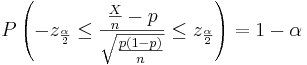
Let be a random sample from the Bernoulli distribution with probability of success p. To construct a confidence interval for p the following result is used based on normal approximation: 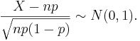 Therefore,
-
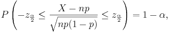
- where and defined as above.
After rearranging we get:
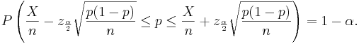
The ratio  is the point estimate of the population p and it is denoted with
  . The problem with this interval is that the unknown p appears also at the end points of the interval. As an approximation we can simply replace p with its estimate . Finally the confidence interval is given by:
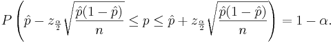
We say that we are 1 − α confident that p falls in 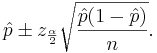
Calculating sample sizes
The basic problem we will address now is how to determine the sample size needed so that the resulting confidence interval will have a fixed margin of error E with confidence level 1 − α.
In the expression 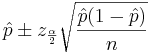 , the width of the confidence interval is given by the margin of error
  . We can simply solve for n:
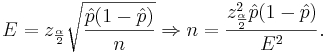
However, the value of  is not known because we have not observed our sample yet. If we use
  , we will obtain the largest possible sample size. Of course, if we have an idea about its value (from another study, etc.) we can use it.
Example 6
At a survey poll before the elections candidate A receives the support of 650 voters in a sample of 1,200 voters.
- Construct a 95% confidence interval for the population proportion p that supports candidate A.
- Find the sample size needed so that the margin of error will be
 with confidence level 95%.
Another formula for the confidence interval for the population proportion p
Another way to solve for p is presented below:

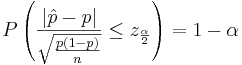
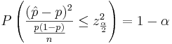
We obtain a quadratic expression in terms of p:
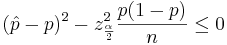
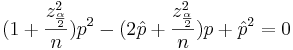
Solving for p we get the following confidence interval:
-
 When n is large, this interval is the same as before.</math>
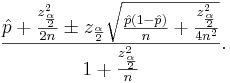
Exact confidence interval for p
The first interval for proportions above (normal approximation) produces intervals that are too narrow when the sample size is small. The coverage is below 1 − α. The following exact method (or Clopper-Pearson) improves the low coverage of the normal approximation confidence interval. The exact confidence interval however has higher coverage than 1 − α.
![\left[1+\frac{n-x+1}{xF_{1-\frac{\alpha}{2};2x,2(n-x+1)}}\right]^{-1} < p <
\left[1+\frac{n-x}{(x+1)F_{\frac{\alpha}{2};2(x+1),2(n-x)}}\right]^{-1},](/socr/uploads/math/d/c/c/dcc9e8ffb611a5d9291ed1a8f0b0b0b8.png)
- where, x is the number of successes among n trials, and Fa,b,c is the a quantile of the F distribution with numerator degrees of freedom b and denominator degrees of freedom c.
Confidence interval for the population variance σ2 of normal distribution
Again, let random sample from N(μ,σ2). It is known that 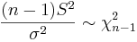 . Therefore,
- where
 and
and  are defined as follows:

As with the T-distribution, the values of and may be found from:
- Interactive SOCR Chi-Square Distribution applet, or
- the SOCR Chi-Square Table. Some examples are included below:
| 1 − α | n | |
|
|---|---|---|---|
| 0.90 | 4 | 0.352 | 7.81 |
| 0.95 | 16 | 6.26 | 27.49 |
| 0.98 | 25 | 10.86 | 42.98 |
| 0.99 | 41 | 20.71 | 66.77 |
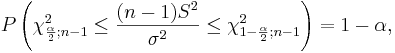
If we rearrange the inequality above we get:
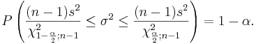
We say that we are 1 − α confident that the population variance σ2 falls in the interval:
![\left[\frac{(n-1)s^2}{\chi_{1-\frac{\alpha}{2};n-1}^2},
\frac{(n-1)s^2}{\chi_{\frac{\alpha}{2};n-1}^2}\right]](/socr/uploads/math/7/c/0/7c0f0a9303215d1243ea7a2bc5c4cc3e.png)
- Comment: When the sample size n is large, the
 distribution can be approximated by
 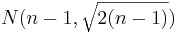 . Therefore, in such situations, the confidence interval for the variance can be computed as follows:
Example 7
A precision instrument is guaranteed to read accurately to within 2 units. A sample of 4 instrument readings on the same object yielded the measurements 353, 351, 351, and 355. Find a 90% confidence interval forn the population variance. Assume that these observations were selected from a population that follows the normal distribution.
SOCR investigation
Using the SOCR confidence intervals applet, we run the following simulation experiment: normal distribution with mean 5 and standard deviation 2, sample size 30, confidence intervals 50, and confidence level 0.95.


However, if the population is not normal, the coverage is poor and this can be seen with the following SOCR example. Consider the exponential distribution with λ = 2 (variance is σ2 = 0.25). If we use the confidence interval based on the χ2 distribution, as described above, we obtain the following results (first with sample size 30 and then sample size 300).


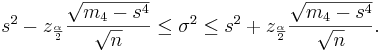
We observe that regardless of the sample size the 95% CI(σ2) coverage is poor. In these situations, (sampling from non-normal populations) an asymptotically distribution-free confidence interval for the variance can be obtained using the following large sample theory result:
-
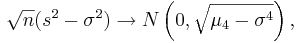
- That is,
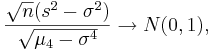
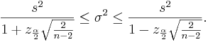
- where, μ4 = E(X − μ)4 is the fourth moment of the distribution. Of course, μ4 is unknown and will be estimated by the fourth sample moment
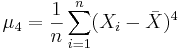 . The confidence interval for the population variance is computed as follows:
Using the SOCR CI Applet, with exponential distribution (λ = 2), sample size 300, number of intervals 50, confidence level 0.95) we see that the coverage of this interval is approximately 95%.


The 95% CI(σ2) coverage for the intervals constructed using the method of asymptotic distribution-free intervals is much closer to 95%.
Confidence intervals for the population parameters of a distribution based on the asymptotic properties of maximum likelihood estimates
To construct confidence intervals for parameter of a distribution the following method can be used based on the large sample theory of maximum likelihood estimates. As the sample size n increases it can be shown that the maximum likelihood estimate  of a parameter θ follows approximately normal distribution with mean θ and variance equal to the lower bound of the Cramer-Rao inequality.

Because I(θ) (Fisher's information) is a function of the unknown parameter θ we replace θ with its maximum likelihood estimate to get  .
.
Since, 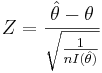 , we can write
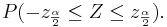 If we replace Z with , we get
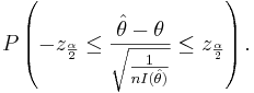
Therefore,
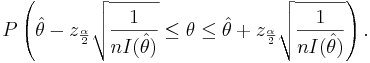
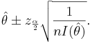
Thus, we are 1 − α confident that θ falls in the interval
Example 8
Use the result above to construct a confidence interval for the Poisson parameter \lambda. Let be independent and identically distributed random variables from a Poisson distribution with parameter λ.
We know that the maximum likelihood estimate of λ is  . We need to find the lower bound of the Cramer-Rao inequality:
 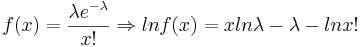 .
.
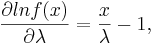
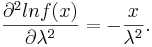
Let's find the first and second derivatives w.r.t. λ.
Therefore, 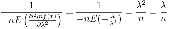 . When n is large,
  follows approximately
 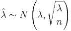 . Because λ is unknown, we replace it with its MLE estimate :
-
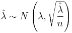
- or
Therefore, the confidence interval for λ is:
Application
The number of pine trees at a certain forest follows the Poisson distribution with unknown parameter λ per acre. A random sample of size n=50 acres is selected and the number of pine trees in each acre is counted. Here are the results:
7 4 5 3 1 5 7 6 4 3 2 6 6 9 2 3 3 7 2 5 5 4 4 8 8 7 2 6 3 5 0
5 8 9 3 4 5 4 6 1 0 5 4 6 3 6 9 5 7 6
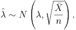
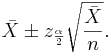
The sample mean is  . Therefore, a 95% confidence interval for the parameter λ is
-
- That is,
Therefore  .
.
Exponential distribution
Verify that for the parameter λ of the exponential distribution the confidence interval obtained by this method is given as follows:
The following SOCR simulations refer to
- Poisson distribution, λ = 5, sample size 40, number of intervals 50, confidence level 0.95.


- Exponential distribution, λ = 0.5, sample size 30, number of intervals 50, confidence level 0.95.


References
- Mega, M., Dinov, I., Thompson, P., Manese, M., Lindshield, C., Moussai, J., Tran, N., Olsen, K., Felix, J., Zoumalan, C., Woods, R., Toga, A., and Mazziotta, J. (2005). Automated brain tissue assessment in the elderly and demented population: Construction and validation of a sub-volume probabilistic brain atlas. NeuroImage, 26(4), 1009-1018.
- Stewarty, C. (1999). Robust Parameter Estimation in Computer Vision. SIAM Review, 41(3), 513–537.
- Wolfram, S. (2002). A New Kind of Science, Wolfram Media Inc.
- Agresti A, Coull A. “Approximate is Better than Exact for Interval Estimation of Binomial Proportions” American Statistician (1998).
- Sauro, J., Lewis, J. R., Estimating Completion Rates From Small Samples Using Binomial Confidence Intervals: Comparisons and Recommendations, Proceedings of the Human Factor AND Ergonomics Society 49th Annual Meeting (2005).
- Hogg, R. V., Tanis, E. A., Probability and Statistical Inference, 3rd Edition, Macmillan (1988).
- Ferguson, T., S., A Course in Large Sample Theory, Chapman & Hall (1996).
- John Rice, Mathematical Statistics and Data Analysis, Third Edition, Duxbury Press (2006).
Translate this page:
