SOCR EduMaterials Activities ParetoEstimateExperiment
From Socr
Contents |
Pareto Estimate Experiment
Description
The experiment is to generate a random sample X1,X2,...,Xn of size n from the Pareto distribution with (power) parameter a. The distribution density is shown in blue in the graph, and on each update, the sample density is shown in red. One each update, the following statistics are recorded:
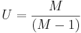 , where
 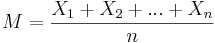 and
and
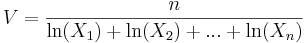 Statistics U and V are point estimators of a. As the experiment runs, the empirical bias and mean square error of each estimator are recorded in the second table. The parameters a and n can be varied with scroll bars.
Goal
To provide a simulation demonstrating properties of the Pareto distribution that deals with continuous probability distributions. In addition, the Pareto distribution is relative to the exponential distribution as well as the gamma distribution so after experimenting with this applet, users should be able to develop a generalization for these three types of distributions.
Experiment
Go to the SOCR Experiments and select the Pareto Estimate Experiment from the drop-down list of experiments on the top left. The image below shows the initial view of this experiment:

When pressing the play button, one trial will be executed and recorded in the distribution table below. The fast forward button symbolizes the nth number of trials to be executed each time. The stop button ceases any activity and is helpful when the experimenter chooses “continuous,” indicating an infinite number of events. The fourth button will reset the entire experiment, deleting all previous information and data collected.
The “update” scroll indicates nth number of trials (1, 10, 100, or 1000) performed when selecting the fast forward button and the “stop” scroll indicates the maximum number of trials in the experiment.
Since parameter a may be varied according to the user, the smaller the value, the more skewed right the distribution graph will be. When a consists a large value, it is still skewed right but the distribution graph is less curved. The image below shown below demonstrates both changes in a:


Note that the empirical density and moments graph begin to converge to the distribution graph after every trial. In other words, the empirical graph is more saturated at the left side of the graph because the distribution graph obtains maximum values on this side. The spread of the empirical graph is rather large but most of the values are towards the left with outliers on the right. The image shown below demonstrates this:

Applications
The Pareto Estimate Experiment is an applet that generalizes the important of experiments involving continuous probability distributions. It may be used in many different types of examples:
Suppose contractors want to find out the mean, median, and mode as well as the characteristics of the probability density function of the sizes of sand particles at their work site.
Scientists obtained numbers of species per genus and want to gather all data information to develop a probability density graph that will represent their findings.
Environmentalists want to prevent forest fires so they are interested in developing a representation for all the areas burnt from forest fires to illustrate which field of study should be their main focus.
Translate this page:
