SOCR EduMaterials Activities RNG
From Socr
(→Applications) |
|||
| (14 intermediate revisions not shown) | |||
| Line 1: | Line 1: | ||
| - | == [[SOCR_EduMaterials_Activities | SOCR Educational Materials - Activities]] - SOCR Random | + | == [[SOCR_EduMaterials_Activities | SOCR Educational Materials - Activities]] - SOCR Random Number Generation (RNG) Activity == |
| - | + | == Summary== | |
| - | This activity describes the need, general methods and SOCR utilities for random number generation and simulation. [http://www.socr.ucla.edu/htmls/SOCR_Modeler.html SOCR Modeler] allows interactive sampling from any [[About_pages_for_SOCR_Distributions | SOCR Distribution]]. | + | This activity describes the need, general methods and SOCR utilities for random number generation and simulation. [http://www.socr.ucla.edu/htmls/SOCR_Modeler.html SOCR Modeler] allows interactive sampling from any [[About_pages_for_SOCR_Distributions | SOCR Distribution]]. The simulated data may then be easily copied and pasted in different SOCR [http://www.socr.ucla.edu/htmls/SOCR_Analyses.html Analyses] or [http://www.socr.ucla.edu/htmls/SOCR_Charts.html Graphing] tools for further interrogation. |
| - | + | ==Goals== | |
The aims of this activity are to: | The aims of this activity are to: | ||
* motivate the need for robust random number generators | * motivate the need for robust random number generators | ||
| Line 10: | Line 10: | ||
* present applications of random number generation | * present applications of random number generation | ||
| - | + | ==Background & Motivation== | |
| - | '''How many natural processes or phenomena in real life can you describe that have an exact mathematical close-form description and are completely deterministic?''' Arrival | + | '''How many natural processes or phenomena in real life can you describe that have an exact mathematical close-form description and are completely deterministic?''' Arrival times to school each day? Motion of the Moon around the Earth? The computer CPU? The atomic clock? It is an unsettling paradox that all natural phenomena we observe are stochastic in nature. Yet, we do not know how to replicate any of them exactly. There are good computational strategies to approximate natural processes using analytical mathematical models; however, upon careful review one always finds out a deterministic pattern in all purely computationally generated processes. |
| - | '''There are two strategies to generate random numbers.''' The first one relies on a ''physical process'' which is expected to be random. The other uses ''computational algorithms'' that produce long sequences of apparently random results, which are in fact determined by a shorter initial seed. Random number generators based on ''physical processes'' may be based on random particles' momentum or position or any of the [http://en.wikipedia.org/wiki/GUT three fundamental physical forces]. Examples of such | + | '''There are two strategies to generate random numbers.''' The first one relies on a ''physical process'' which is expected to be random. The other uses ''computational algorithms'' that produce long sequences of apparently random results, which are in fact determined by a shorter initial seed. Random number generators based on ''physical processes'' may be based on random particles' momentum or position or any of the [http://en.wikipedia.org/wiki/GUT three fundamental physical forces]. Examples of such processes are the Atari gaming console (noise from an analog circuits to generate true random numbers), radioactive decay, thermal noise, shot noise and clock drift. A random number generator (RNG) based solely on deterministic computation is referred to ''pseudo-random number generator''. There are [http://en.wikipedia.org/wiki/Random_number_generator various techniques for obtaining computational (pseudo)random numbers]. Virtually all RNG's used in practice are pseudo-RNGs. To distinguish real random numbers from the pseudo-random numbers is a very difficult problem. |
'''If all natural processes are inherently random and at the same time we can not generate ourselves good (non-deterministic) RNG processes why are we even attempting to do that?''' Wouldn't it be much easier to just use measurements of the natural physical processes? The answer is simple: We typically need to sample/simulate data from a ''specific process'' and it is not easy to show that a physical phenomena we observe has the same distribution as the process of interest! So, our need of sampling from a specific distribution demands that we ensure the proper characteristics of the sample. | '''If all natural processes are inherently random and at the same time we can not generate ourselves good (non-deterministic) RNG processes why are we even attempting to do that?''' Wouldn't it be much easier to just use measurements of the natural physical processes? The answer is simple: We typically need to sample/simulate data from a ''specific process'' and it is not easy to show that a physical phenomena we observe has the same distribution as the process of interest! So, our need of sampling from a specific distribution demands that we ensure the proper characteristics of the sample. | ||
| - | '''Where does this sampling need come from?''' Random number generators have several important applications in statistical modeling, computer simulation, cryptography, etc. For example, data collection is often very expensive. Hence, to do appropriate inference on datasets of smaller sizes, we may consider simulating repeatedly from appropriate distributions, instead of using real observations. Another example of why are random number generators so important comes from cryptography. It is a commonly held misconception that every encryption method can be broken. Claude Shannon, Bell Labs, 1948, proved that the [http://en.wikipedia.org/wiki/One-time_pad one-time pad cipher] is unbreakable, provided the secret key is truly random and of length equal or greater than the length of the encoded message. [http://en.wikipedia.org/wiki/Monte_carlo_simulation Monte Carlo simulations] are also based on RNGs and are used for finding numerical solutions to (multi-dimensional) mathematical problems that cannot easily be solved exactly. For example, integration, differentiation, root-finding, etc. | + | '''Where does this sampling-need come from?''' Random number generators have several important applications in statistical modeling, computer simulation, cryptography, etc. For example, data collection is often very expensive. Hence, to do appropriate inference on datasets of smaller sizes, we may consider simulating repeatedly from appropriate distributions, instead of using real observations. Another example of why are random number generators so important comes from cryptography. It is a commonly held misconception that every encryption method can be broken. Claude Shannon, Bell Labs, 1948, proved that the [http://en.wikipedia.org/wiki/One-time_pad one-time pad cipher] is unbreakable, provided the secret key is truly random and of length equal or greater than the length of the encoded message. [http://en.wikipedia.org/wiki/Monte_carlo_simulation Monte Carlo simulations] are also based on RNGs and are used for finding numerical solutions to (multi-dimensional) mathematical problems that cannot easily be solved exactly. For example, integration, differentiation, root-finding, etc. |
| - | + | ==Exercises== | |
| - | + | * '''Exercise 1''': Go to the [http://www.socr.ucla.edu/htmls/SOCR_Modeler.html SOCR Modeler] and click on the '''Data Generation''' tab. Select 200 observations from the [http://wiki.stat.ucla.edu/socr/index.php/About_pages_for_SOCR_Distributions Generalized Beta Distribution], as shown on the image below. Choose this four-tuple for the parameters <math> \alpha=1.5; \beta=3; A=0; B=7</math>. Copy these 200 values in your mouse buffer (CNT-C) and paste them in the '''Data''' tab of the '''LineCharts --> PowerTransformHistogramChart''' under [http://www.socr.ucla.edu/htmls/SOCR_Charts.html SOCR Charts]. Then ''Map'' this column to ''XYValue'' (under the '''MAP''' tab) and click '''Update_Chart'''. This will generate the histogram of the 200 observations. Indeed, this graph should look like a discrete analog of the [http://wiki.stat.ucla.edu/socr/index.php/About_pages_for_SOCR_Distributions Generalized Beta] density curve. You can see exactly what the [http://wiki.stat.ucla.edu/socr/index.php/About_pages_for_SOCR_Distributions Generalized Beta Distribution] looks like by going to [http://www.socr.ucla.edu/htmls/SOCR_Distributions.html SOCR Distributions] and selecting <math> Beta(\alpha=1.5; \beta=3; A=0; B=7)</math>. | |
| - | * Go to the [http://www.socr.ucla.edu/htmls/SOCR_Modeler.html SOCR Modeler] and click on the '''Data Generation''' tab. Select 200 observations from the [http://wiki.stat.ucla.edu/socr/index.php/About_pages_for_SOCR_Distributions Generalized Beta Distribution], as shown on the image below. Choose this four-tuple for the parameters <math> \alpha=1.5; \beta=3; A=0; B=7</math>. Copy these 200 values in your mouse buffer (CNT-C) and paste them in the '''Data''' tab of the '''LineCharts --> PowerTransformHistogramChart''' under [http://www.socr.ucla.edu/htmls/SOCR_Charts.html SOCR Charts]. Then ''Map'' this column to ''XYValue'' (under the '''MAP''' tab) and click '''Update_Chart'''. This will generate the histogram of the 200 observations. Indeed, this graph should look like a discrete | + | |
<center>[[Image:SOCR_Activities_PowerTransformGraphing_Dinov_022007_Fig10.jpg|400px]] | <center>[[Image:SOCR_Activities_PowerTransformGraphing_Dinov_022007_Fig10.jpg|400px]] | ||
| Line 27: | Line 26: | ||
</center> | </center> | ||
| - | * | + | * '''Exercise 2''': Let’s get some more simulated data: Go to [http://www.socr.ucla.edu/htmls/SOCR_Modeler.html SOCR Modeler] and generate 100 Cauchy Distributed variables. Copy these data in your mouse buffer (CNT-C). Of course, you may choose any other distribution. Next, paste (CNT-V) these 100 observations in [http://www.socr.ucla.edu/htmls/SOCR_Charts.html SOCR Charts] ('''Line-Charts -> Power Transform Chart'''). ''Map'' this column to ''XYValue'' (under the '''MAP''' tab) and click '''Update_Chart''' to see the index plot of this data in RED! |
| - | + | <center>[[Image:SOCR_Activities_PowerTransformGraphing_Dinov_022007_Fig1.jpg|400px]] | |
| - | + | [[Image:SOCR_Activities_PowerTransformGraphing_Dinov_022007_Fig2.jpg|400px]]</center> | |
| - | + | Imagine now that we want to compare the bell-shape-looking [[About_pages_for_SOCR_Distributions | Cauchy]] and [[About_pages_for_SOCR_Distributions | Normal]] distributions. As pointed out above, we can generate 1,000 random Cauchy observations (using the '''Data Generation''' tab of the [http://socr.ucla.edu/htmls/SOCR_Modeler.html SOCR Modeler]). Then we can fit the best possible Normal distribution to the histogram of these 1,000 Cauchy observations. As the figure below shows the best ([http://en.wikipedia.org/wiki/Maximum_likelihood maximum likelihood estimates]) for the mean and variance of the best normal fit are ''(-0.8529654842885793, 6355.713457104439)''. The measure of centrality (mean) is pretty accurately estimated (exact center of Cauchy is zero (Cauchy is symmetric), even though its mean is undefined). The variance is large, as Cauchy distribution has much heavier tails than Normal distribution -- hence it's ''Bell-Shapeness'' is '''misleading'''! The distribution insert on the right illustrates the exact Cauchy distribution, which you can see interactively in [http://socr.ucla.edu/htmls/SOCR_Distributions.html SOCR Distributions]. | |
| - | + | <center>[[Image:SOCR_Activities_PowerTransformGraphing_Dinov_091707_Fig3.jpg|400px]]</center> | |
| - | + | ||
| - | + | ||
| - | + | ||
| - | + | ||
| - | <center>[[Image: | + | |
| - | + | ||
| - | + | ||
| - | + | ||
| - | + | ||
| - | + | ||
| - | + | ||
| - | + | ||
| - | + | ||
| - | + | ||
| - | + | ||
| - | + | ||
| - | <center>[[Image: | + | |
| - | + | ||
| - | + | ||
| - | + | ==Applications== | |
| - | The | + | The RNG background and motivation section clearly described some of the critical scientific and technological challenges that rely upon the existence of quality RNGs. Here we present the applications of the SOCR RNG's for various interactive activities and demonstrations. |
* [[SOCR_EduMaterials_Activities_PowerTransformFamily_Graphs | Power-Transform Family Graphs]] | * [[SOCR_EduMaterials_Activities_PowerTransformFamily_Graphs | Power-Transform Family Graphs]] | ||
| - | * | + | * [http://wiki.stat.ucla.edu/socr/index.php/SOCR_EduMaterials_ModelerActivities_MixtureModel_1 Mixture Model Experiment] |
Current revision as of 01:26, 3 May 2008
Contents |
SOCR Educational Materials - Activities - SOCR Random Number Generation (RNG) Activity
Summary
This activity describes the need, general methods and SOCR utilities for random number generation and simulation. SOCR Modeler allows interactive sampling from any SOCR Distribution. The simulated data may then be easily copied and pasted in different SOCR Analyses or Graphing tools for further interrogation.
Goals
The aims of this activity are to:
- motivate the need for robust random number generators
- illustrate how to use the SOCR random number generators
- present applications of random number generation
Background & Motivation
How many natural processes or phenomena in real life can you describe that have an exact mathematical close-form description and are completely deterministic? Arrival times to school each day? Motion of the Moon around the Earth? The computer CPU? The atomic clock? It is an unsettling paradox that all natural phenomena we observe are stochastic in nature. Yet, we do not know how to replicate any of them exactly. There are good computational strategies to approximate natural processes using analytical mathematical models; however, upon careful review one always finds out a deterministic pattern in all purely computationally generated processes.
There are two strategies to generate random numbers. The first one relies on a physical process which is expected to be random. The other uses computational algorithms that produce long sequences of apparently random results, which are in fact determined by a shorter initial seed. Random number generators based on physical processes may be based on random particles' momentum or position or any of the three fundamental physical forces. Examples of such processes are the Atari gaming console (noise from an analog circuits to generate true random numbers), radioactive decay, thermal noise, shot noise and clock drift. A random number generator (RNG) based solely on deterministic computation is referred to pseudo-random number generator. There are various techniques for obtaining computational (pseudo)random numbers. Virtually all RNG's used in practice are pseudo-RNGs. To distinguish real random numbers from the pseudo-random numbers is a very difficult problem.
If all natural processes are inherently random and at the same time we can not generate ourselves good (non-deterministic) RNG processes why are we even attempting to do that? Wouldn't it be much easier to just use measurements of the natural physical processes? The answer is simple: We typically need to sample/simulate data from a specific process and it is not easy to show that a physical phenomena we observe has the same distribution as the process of interest! So, our need of sampling from a specific distribution demands that we ensure the proper characteristics of the sample.
Where does this sampling-need come from? Random number generators have several important applications in statistical modeling, computer simulation, cryptography, etc. For example, data collection is often very expensive. Hence, to do appropriate inference on datasets of smaller sizes, we may consider simulating repeatedly from appropriate distributions, instead of using real observations. Another example of why are random number generators so important comes from cryptography. It is a commonly held misconception that every encryption method can be broken. Claude Shannon, Bell Labs, 1948, proved that the one-time pad cipher is unbreakable, provided the secret key is truly random and of length equal or greater than the length of the encoded message. Monte Carlo simulations are also based on RNGs and are used for finding numerical solutions to (multi-dimensional) mathematical problems that cannot easily be solved exactly. For example, integration, differentiation, root-finding, etc.
Exercises
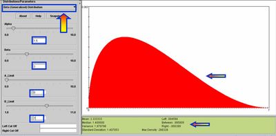
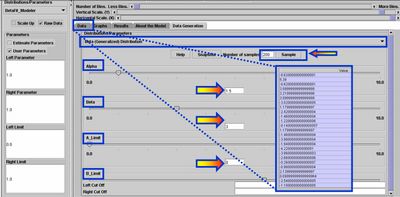
- Exercise 1: Go to the SOCR Modeler and click on the Data Generation tab. Select 200 observations from the Generalized Beta Distribution, as shown on the image below. Choose this four-tuple for the parameters α = 1.5;β = 3;A = 0;B = 7. Copy these 200 values in your mouse buffer (CNT-C) and paste them in the Data tab of the LineCharts --> PowerTransformHistogramChart under SOCR Charts. Then Map this column to XYValue (under the MAP tab) and click Update_Chart. This will generate the histogram of the 200 observations. Indeed, this graph should look like a discrete analog of the Generalized Beta density curve. You can see exactly what the Generalized Beta Distribution looks like by going to SOCR Distributions and selecting Beta(α = 1.5;β = 3;A = 0;B = 7).
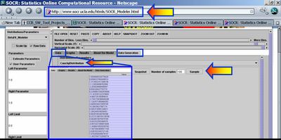
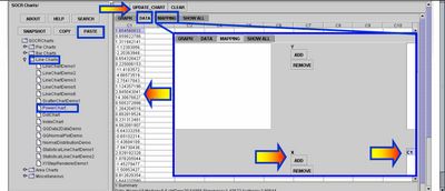
- Exercise 2: Let’s get some more simulated data: Go to SOCR Modeler and generate 100 Cauchy Distributed variables. Copy these data in your mouse buffer (CNT-C). Of course, you may choose any other distribution. Next, paste (CNT-V) these 100 observations in SOCR Charts (Line-Charts -> Power Transform Chart). Map this column to XYValue (under the MAP tab) and click Update_Chart to see the index plot of this data in RED!
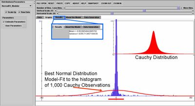
Imagine now that we want to compare the bell-shape-looking Cauchy and Normal distributions. As pointed out above, we can generate 1,000 random Cauchy observations (using the Data Generation tab of the SOCR Modeler). Then we can fit the best possible Normal distribution to the histogram of these 1,000 Cauchy observations. As the figure below shows the best (maximum likelihood estimates) for the mean and variance of the best normal fit are (-0.8529654842885793, 6355.713457104439). The measure of centrality (mean) is pretty accurately estimated (exact center of Cauchy is zero (Cauchy is symmetric), even though its mean is undefined). The variance is large, as Cauchy distribution has much heavier tails than Normal distribution -- hence it's Bell-Shapeness is misleading! The distribution insert on the right illustrates the exact Cauchy distribution, which you can see interactively in SOCR Distributions.
Applications
The RNG background and motivation section clearly described some of the critical scientific and technological challenges that rely upon the existence of quality RNGs. Here we present the applications of the SOCR RNG's for various interactive activities and demonstrations.
- SOCR Home page: http://www.socr.ucla.edu
Translate this page:
