SOCR EduMaterials ModelerActivities NormalBetaModelFit
From Socr
Contents |
SOCR Educational Materials - Activities - SOCR Normal and Beta Distribution Model Fit Activity
Summary
This activity describes the process of SOCR model fitting in the case of using Normal or Beta distribution models. Model fitting is the process of determining the parameters for an analytical model in usch a way that we obtain optimal parameter estimates according to some critirion. There are many strategies for parameter estimation. The differences between most of these are the underlying cost-functions and the optimization strategies applied to maximize/minimize the cost-function.
Goals
The aims of this activity are to:
- motivate the need for (analytical) modeling of natural processes
- illustrate how to use the SOCR Modeler to fit models to real data
- present applications of model fitting
Background & Motivation
Suppose we are given the sequence of numbers {1, 2, 3, 4, 5, 6, 7, 8, 9, 10} and asked to find the best (Continuous) Uniform Distribution that fits that data. In this case there are two parameters that need to be estimated - the minimum (m) and the maximum (M) of the data. These parameters determine exactly the support (domain) of the continuous distribution and we can explicitely write the density for the (best fit) continuous uniform distribution as:
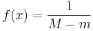 , for
, for 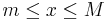 and f(x) = 0, for
 ![x \notin [m:M]](/socr/uploads/math/e/e/e/eeebe52f24cd83c54aa66942a5904c29.png) .
.Having this model distribution, we can use it's analytical form (f(x))to compute probabilities of events, critical functional values and, in general, do inference on the native process withiout acquirying additional data. Hence a good strategy for model fitting is extremely useful in data analysis and statitical inference. Of course, any inference based on models is only going to be as good as the data and the optimization strategy used to generate the model.
Let's look at another motivational example. This time, suppose we have recorded the following measurements from a procces {1.2, 1.7, 3.4, 1.5, 1.1, 1.7, 3.5, 2.5}. Taking bin-size of 1, we can easily calculate the frequency histogram for this process as {6, 1, 2}.

We can now ask about the best Beta distribution model fit to the histogram of the data!
Exercises
Exercise 1
Go to the SOCR Modeler and click on the Data Generation tab. Select 200 observations from the Generalized Beta Distribution, as shown on the image below. Choose this four-tuple for the parameters α = 1.5;β = 3;A = 0;B = 7. Copy these 200 values in your mouse buffer (CNT-C) and paste them in the Data tab of the LineCharts --> PowerTransformHistogramChart under SOCR Charts. Then Map this column to XYValue (under the MAP tab) and click Update_Chart. This will generate the histogram of the 200 observations. Indeed, this graph should look like a discrete analog of the Generalized Beta density curve. You can see exactly what the Generalized Beta Distribution looks like by going to SOCR Distributions and selecting Beta(α = 1.5;β = 3;A = 0;B = 7).
![]()
Applications
TBD
- SOCR Home page: http://www.socr.ucla.edu
Translate this page:
