AP Statistics Curriculum 2007 EDA Var
From Socr
Contents |
General Advance-Placement (AP) Statistics Curriculum - Measures of Variation
Measures of Variation and Dispersion
There are many measures of (population or sample) variation, e.g., the range, the variance, the standard deviation, mean absolute deviation, etc. These are used to assess the dispersion or spread of the population.
Suppose we are interested in the long-jump performance of some students. We can carry an experiment by randomly selecting eight male statistics students and ask them to perform the standing long jump. In reality every student participated, but for the ease of calculations below we will focus on these eight students. The long jumps were as follows:
| 60 | 64 | 68 | 74 | 76 | 78 | 80 | 106 |
Range
The range is the easiest measure of dispersion to calculate, yet, perhaps not the best measure. The Range = max - min. For example, for the Long Jump data, the range is calculated by:
Note that the range is only sensitive to the extreme values of a sample and ignores all other information. So, two completely different distributions may have the same range.
Quartiles and IQR
The first quartile (Q1) and the third quartile (Q3) are defined values that split the dataset into bottom-25% vs. top-75% and bottom-75% vs. top-25%, respectively. Thus the inter-quartile range (IQR), which is the difference Q3 − Q1, represents the central 50% of the data and can be considered as a measure of data dispersion or variation. The wider the IQR, the more variant the data.
For example, Q1 = (64 + 68) / 2 = 66, Q3 = (78 + 80) / 2 = 79 and IQR = Q3 − Q1 = 13, for the Long-Jump data shown above. Thus we expect the middle half of all long jumps (for that population) to be between 66 and 79 inches.
Coefficient of Variation
For a given process, the coefficient of variation (CV) is defined as the ratio of the standard deviation (σ) to the mean (μ):

Obviously, the CV is well-defined for processes with well-defined first two moments (mean and variance), but also requires a non-trivial mean ( ). If the CV is expressed as percentage, than this ratio is multiplied by 100. The sample coefficient of variation is computed mostly for data measured on a ratio scale. For instance, if a set of distances are measured, the standard deviation does not depend on whether the distances were measured in kilometers (metric) or miles. This is because changes in the particle/object's distances by 1 kilometer also changes its distance by 1 mile. However the mean distance of the data would differ in each measurement scale (as 1 mile is approximately 1.7 kilometers) and thus the coefficient of variation would differ. In general, the CV may not have any meaning for data on an interval scale.
The sample-coefficient of variation is computed by plugin the sample-driven estimates of the standard deviation (sample-standard deviation, s, and the sample-average,  ). In image processing, the reciprocal of the coefficient of variation is μ/σ is called signal-to-noise-ratio (SNR).
Five-number summary
The five-number summary for a dataset is the 5-tuple {min,Q1,Q2,Q3,max}, containing the sample minimum, first-quartile, second-quartile (median), third-quartile, and maximum.
Variance and Standard Deviation
The logic behind the variance and standard deviation measures is to measure the difference between each observation and the mean (i.e., dispersion). Suppose we have n > 1 observations,  . The deviation of the ith measurement, yi, from the mean (
 ) is defined by
  .
.
Does the average of these deviations seem like a reasonable way to find an average deviation for the sample or the population? No, because the sum of all deviations is trivial:
To solve this problem we employ different versions of the mean absolute deviation:
In particular, the variance is defined as:
And the standard deviation is defined as:
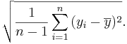
For the long-jump sample of 8 measurements, the standard deviation is:

Activities
Try to pair each of the 4 samples whose numerical summaries are reported below with one of the 4 frequency plots below. Explain your answers.
| Sample | Mean | Median | StdDev |
| A | 4.688 | 5.000 | 1.493 |
| B | 4.000 | 4.000 | 1.633 |
| C | 3.933 | 4.000 | 1.387 |
| D | 4.000 | 4.000 | 2.075 |

Notes
- Some software packages may use
 , instead of the
  , which we used above. Note that for large sample-sizes this difference becomes increasingly smaller. Also, there are theoretical properties of the sample variance, as defined above (e.g., sample-variance is an unbiased estimate of the population-variance!)
- Most of the SOCR Charts and SOCR Analyses compute the variance or standard deviation for the sample. You can see these examples of Charts Activities and Analyses Activities and you can test these using hotdogs dataset.
Problems
References
- SOCR Home page: http://www.socr.ucla.edu
Translate this page:
