AP Statistics Curriculum 2007 GLM MultLin
From Socr
Contents |
General Advance-Placement (AP) Statistics Curriculum - Multiple Linear Regression
In the previous sections, we saw how to study the relations in bivariate designs. Now we extend that to any finite number of variables (multivariate case).
Multiple Linear Regression
We are interested in determining the linear regression, as a model, of the relationship between one dependent variable Y and many independent variables Xi, i = 1, ..., p. The multilinear regression model can be written as
-
 , where
  is the error term.
The coefficient β0 is the intercept ("constant" term) and βis are the respective parameters of the p independent variables. There are p+1 parameters to be estimated in the multilinear regression.
- Multilinear vs. non-linear regression: This multilinear regression method is "linear" because the relation of the response (the dependent variable Y) to the independent variables is assumed to be a linear function of the parameters βi. Note that multilinear regression is a linear modeling technique not because that the graph of Y = β0 + βx is a straight line nor because Y is a linear function of the X variables. But the "linear" term refers to the fact that Y can be considered a linear function of the parameters ( βi), even though it is not a linear function of X. Thus, any model like
-
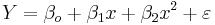
is still one of the linear regression, that is, linear in x and x2 respectively, even though the graph on x by itself is not a straight line.
Parameter Estimation in Multilinear Regression
A multilinear regression with p coefficients and the regression intercept β0 and n data points (sample size), with 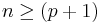 allows construction of the following vectors and matrix with associated standard errors:
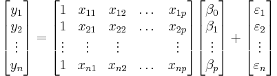
or, in vector-matrix notation
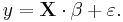
Each data point can be given as  ,
,  . For n = p, standard errors of the parameter estimates could not be calculated. For n less than p, parameters could not be calculated.
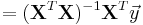
- Point Estimates: The estimated values of the parameters βi are given as

- Residuals: The residuals, representing the difference between the observations and the model's predictions, are required to analyse the regression and are given by:
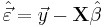
The standard deviation,  for the model is determined from
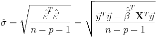
The variance in the errors is Chi-square distributed:
- Interval Estimates: The 100(1 − α)% confidence interval for the parameter, βi, is computed as follows:
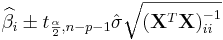 ,
,
where t follows the Student's t-distribution with n − p − 1 degrees of freedom and  denotes the value located in the ith row and column of the matrix.
The regression sum of squares (or sum of squared residuals) SSR (also commonly called RSS) is given by:
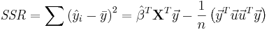 ,
,
where 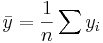 and
and  is an n by 1 unit vector (i.e. each element is 1). Note that the terms yTu and uTy are both equivalent to
  , and so the term
  is equivalent to
  .
.
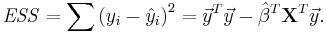
The error (or explained) sum of squares (ESS) is given by:
The total sum of squares (TSS) is given by

Partial Correlations
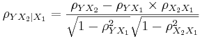
For a given linear model
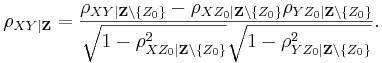
the partial correlation between X1 and Y given a set of p-1 controlling variables  , denoted by
  , is the correlation between the residuals RX and RY resulting from the linear regression of X with Z and that of Y with Z, respectively. The first-order partial correlation is just the difference between a correlation and the product of the removable correlations divided by the product of the coefficients of alienation of the removable correlations.
- Partial correlation coefficients for three variables is calculated from the pairwise simple correlations.
- If,
 ,
,
- then the partial correlation between Y and X2, adjusting for X1 is:
-
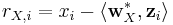
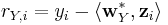
- In general, the sample partial correlation is
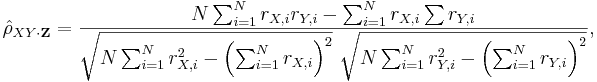 where the residuals rX,i and rX,i are given by:
-
-
 ,
,
- with xi, yi and zi denoting the random (IID) samples of some joint probability distribution over X, Y and Z.
-
Computing the partial correlations
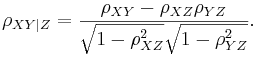
The nth-order partial correlation (|Z| = n) can be computed from three (n - 1)th-order partial correlations. The 0th-order partial correlation  is defined to be the regular correlation coefficient ρYX.
For any  :
:
Implementing this computation recursively yields an exponential time complexity.
Note in the case where Z is a single variable, this reduces to:
Categorical Variables in Multiple Regression
When using categorical variables with more than two levels in a multiple regression modeling, we need to make sure the results are correctly interpreted. For categorical variables with more than 2 levels, a number of separate, dichotomous variables need to be created – this is called “dummy coding” or “dummy variables”.
Dichotomous categorical predictor variables, variables with two levels, may be directly entered as predictor or predicted variables in a multiple regression model. Their use in multiple regression is a direct extension of their use in simple linear regression. The interpretation of their regression weights depends upon how the variables are coded. If dichotomous variables are coded as 0 and 1, their regression weights are added or subtracted to the predicted value of the response variable, Y, depending upon whether it is positive or negative.
If a dichotomous variable is coded as -1 and 1, then if the regression weight is positive, it is subtracted from the group coded as -1 and added to the group coded as 1. If a regression weight is negative, then addition and subtraction is reversed. Dichotomous variables are also included in hypothesis tests for R2 change like any other quantitative variable.
Adding variables to a linear regression model will always increase the (unadjusted) \(R^2\) value. If additional predictor variables are correlated with the predictor variables already in the model, then the combined results may be difficult to predict. In some cases, the combined result will only slightly improve the prediction, whereas in other cases, a much better prediction may be obtained by combining two correlated variables.
If the additional predictor variables are uncorrelated (their correlation is trivial) with the predictor variables already in the model, then the result of adding additional variables to the regression model is easy to predict. Thus, the \(R^2\) change will be equal to the correlation coefficient squared between the added variable and predicted variable. In this case it makes no difference what order the predictor variables are entered into the prediction model. For example, if \(X_1\) and \(X_2\) were uncorrelated \(\rho_{12} = 0\) and \(\rho^2_{1y} = 0.4\) and \(\rho^2_{2y} = 0.5\), then \(R^2\) for \(X_1\) and \(X_2\) would equal \(0.4 + 0.5 = 0.9\). The value for \(R^2\) change for \(X_2\), given that X1 is included in the model, would be 0.5. The value for \(R^2\) change for \(X_2\) given no variable was in the model would be 0.5. It would make no difference at what stage \(X_2\) was entered into the model, the value for \(R^2\) change would always be 0.5. Similarly, the \(R^2\) change value for \(X_1\) would always be 0.4. Because of this relationship, uncorrelated predictor variables will be preferred, when possible.
Look at the Modeling and Analysis of Clinical, Genetic and Imaging Data of Alzheimer’s Disease dataset. It is fairly clear that DX_Conversion could be directly entered into a regression model predicting MMSE, because it is dichotomous. The problem is how to deal with the two categorical predictor variables with more than two levels (e.g., GDTOTAL).
Dummy Coding refers to making many dichotomous variables out of one multilevel categorical variable. Because categorical predictor variables cannot be entered directly into a regression model and be meaningfully interpreted, some other method of dealing with information of this type must be developed. In general, a categorical variable with k levels will be transformed into k-1 variables each with two levels. For example, if a categorical variable had 4 levels, then 3 dichotomous (dummy) variables could be constructed that would contain the same information as the single categorical variable. Dichotomous variables have the advantage that they can be directly entered into the regression model. The process of creating dichotomous variables from categorical variables is called dummy coding.
Depending upon how the dichotomous variables are constructed, additional information can be gleaned from the analysis. In addition, careful construction will result in uncorrelated dichotomous variables. These variables have the advantage of simplicity of interpretation and are preferred to correlated predictor variables.
For example, when using dummy coding with three levels, the simplest case of dummy coding is when the categorical variable has three levels and is converted to two dichotomous variables. School in the example data has three levels, 1=Math, 2=Biology, and 3=Engineering. This variable could be dummy coded into two variables, one called Math and one called Biology. If School = 1, then Math would be coded with a 1 and Biology with a 0. If School=2, then Math would be coded with a 0 and Biology would be coded with a 1. If School=3, then both Math and Biology would be coded with a 0. The dummy coding is represented below.
| Subject | Math | Biology | |
| Math | 1 | 1 | 0 |
| Biology | 2 | 0 | 1 |
| Engineering | 3 | 0 | 0 |
See the SOCR Regression analysis and compare it against SOCR ANOVA.
Dummy Coding into Independent Variables, and the selection of an appropriate set of dummy codes, will result in new variables that are uncorrelated or independent of each other. In the case when the categorical variable has three levels this can be accomplished by creating a new variable where one level of the categorical variable is assigned the value of -2 and the other levels are assigned the value of 1. The signs are arbitrary and may be reversed, that is, values of 2 and -1 would work equally well. The second variable created as a dummy code will have the level of the categorical variable coded as -2 given the value of 0 and the other values recoded as 1 and -1. In all cases the sum of the dummy coded variable will be zero.
We can directly interpret each of the new dummy-coded variables, called a contrast, and compare levels coded with a positive number to levels coded with a negative number. Levels coded with a zero are not included in the interpretation.
For example, School in the example data has three levels, 1=Math, 2=Biology, and 3=Engineering. This variable could be dummy coded into two variables, one called Engineering (comparing the Engineering School with the other two Schools) and one called Math_vs_Bio (comparing Math versus Biology schools). The Engineering contrast would create a variable where all members of the Engineering Department would be given a value of -2 and all members of the other two Schools would be given a value of 1. The Math_vs_Bio contrast would assign a value of 0 to members of the Engineering Department, 1 divided by the number of members of the Math Department to member of the Math Department, and -1 divided by the number of members of the Biology Department to members of the Biology Department. The Math_vs_Bio variable could be coded as 1 and -1 for Math and Biology respectively, but the recoded variable would no longer be uncorrelated with the first dummy coded variable (Engineering). In most practical applications, it makes little difference whether the variables are correlated or not, so the simpler 1 and -1 coding is generally preferred. The contrasts are summarized in the following table.
| School | Engineering | Math_vs_Bio | |
| Math | 1 | 1 | 1/N1 = 1/12= 0.0833 |
| Biology | 2 | 1 | -1/N2 = -1/7 = -0.1429 |
| Engineering | 3 | -2 | 0 |
Note that the correlation coefficient between the two contrasts is zero. The correlation between the Engineering contrast and Salary is -.585 with a squared correlation coefficient of .342. This correlation coefficient has a significance level of .001. The correlation coefficient between the Math_vs_Bio contrast and Salary is -.150 with a squared value of .023.
Generate the corresponding SOCR ANOVA table.
Show that the significance level is identical to the value when each contrast was entered last into the regression model. In this case the Engineering contrast was significant and the Math_vs_Bio contrast was not. The interpretation of these results would be that the Engineering Department was paid significantly more than the Math and Biology Schools, but that no significant differences in salary were found between the Math and Biology Schools. If a categorical variable had four levels, three dummy coded contrasts would be necessary to use the categorical variable in a regression analysis. For example, suppose that a researcher at a pain center did a study with 4 groups of four patients each (N is being deliberately kept small). The dependent measure is subjective experience of pain. The 4 groups consisted of 4 different treatment conditions.
| Group | Treatment |
|---|---|
| 1 | None |
| 2 | Placebo |
| 3 | Psychotherapy |
| 4 | Acupuncture |
An independent contrast is a contrast that is not a linear combination of any other set of contrasts. Any set of independent contrasts would work equally well if the end result was the simultaneous test of the five contrasts, as in an ANOVA. One of the many possible examples is presented below.
| Group | C1 | C2 | C3 | C4 | |
| None | 1 | 0 | 0 | 0 | 0 |
| Placebo | 2 | 1 | 0 | 0 | 0 |
| Psychotherapy | 3 | 0 | 1 | 0 | 0 |
| Acupuncture | 4 | 0 | 0 | 1 | 0 |
Application of this dummy coding in a regression model entering all contrasts in a single block would result in an ANOVA table similar to the one obtained using Means, ANOVA, or General Linear Model.
This solution would not be ideal, however, because there is considerable information available by setting the contrasts to test specific hypotheses. The levels of the categorical variable generally dictate the structure of the contrasts. In the example study, it makes sense to contrast the two control groups (1 and 2) with the other four experimental groups (3 and 4). Any two numbers would work, one assigned to groups 1 and 2 and the others assigned to the other four groups, but it is conventional to have the sum of the contrasts equal to zero. One contrast that meets this criterion would be (-2, -2, 1, 1). Generally it is easiest to set up contrasts within subgroups of the first contrast. For example, a second contrast might test whether there are differences between the two control groups. This contrast would appear as (1, -1, 0, 0). As can be seen, this would be a contrast within the experimental treatment groups. Within the non-drug treatment, a contrast comparing Group 3 with Group 4 might be appropriate (0, 0, 1, -1). Combined, the contrasts are given in the following table.
| Group | C1 | C2 | C3 | |
| None | 1 | -2 | 1 | 0 |
| Placebo | 2 | -2 | -1 | 0 |
| Psychotherapy | 3 | 1 | 0 | 1 |
| Acupuncture | 4 | 1 | 0 | 1 |
Equal sample sizes are important as the results are much cleaner when the sample sizes are presumed to be equal. However equal sample size are not common in real applications, even in well-designed experiments. Unequal sample size makes the effects no longer independent. This implies that it makes difference in hypothesis testing when the effects are added into the model, first, middle, or last. The same dummy coding that was applied to equal sample sizes will now be applied to the original data with unequal sample sizes.
Examples
We now demonstrate the use of SOCR Multilinear regression applet to analyze multivariate data.
Earthquake Modeling
This is an example where the relation between variables may not be linear or explanatory. In the simple linear regression case, we were able to compute by hand some (simple) examples. Such calculations are much more involved in the multilinear regression situations. Thus we demonstrate multilinear regression only using the SOCR Multiple Regression Analysis Applet.
Use the SOCR California Earthquake dataset to investigate whether Earthquake magnitude (dependent variable) can be predicted by knowing the longitude, latitude, distance and depth of the quake. Clearly, we do not expect these predictors to have a strong effect on the earthquake magnitude, so we expect the coefficient parameters not to be significantly distinct from zero (null hypothesis). SOCR Multilinear regression applet reports this model:


Multilinear Regression on Consumer Price Index
Using the SOCR Consumer Price Index Dataset we can explore the relationship between the prices of various products and commodities. For example, regressing Gasoline on the following three predictor prices: Orange Juice, Fuel and Electricity illustrates significant effects of all these variables as significant explanatory prices (at α = 0.05) for the cost of Gasoline between 1981 and 2006.


2011 Best Jobs in the US
Repeat the multiliniear regression analysis using hte Ranking Dataset of the Best and Worst USA Jobs for 2011.
Problems
- SOCR Home page: http://www.socr.ucla.edu
Translate this page:
