SOCR EduMaterials Activities GCLT Applications
From Socr
Contents |
SOCR Educational Materials - Activities - Applications of the General Central Limit Theorem (CLT)
This is a component of the activity is based on the SOCR EduMaterials Activities GeneralCentralLimitTheorem.
Goals
The aims of this activity are to demonstrate several practical applications of the general CLT. There are many practical examples of using CLT to solve real-life problems. Here are some examples which may be solved using the SOCR CLT resources.
The SOCR CLT Experiment
First start by readying carefully the SOCR EduMaterials Activities GeneralCentralLimitTheorem. Then go over each of the CLT applications that are worked out in this activity supplement. You may find it useful going back abd forth between these applications and the formal CLT activity.
Application 1 (Poisson)
Suppose a call service center expects to get 20 calls a minute for questions regarding each of 17 different vendors that rely on this call center for handling their calls. What is the probability that in a 1-minute interval they receive less than 300 calls in total?
Let Xi be the random variable representing the number of calls received about the ith vendor within a minute, then  , as Xi is the number of arrivals within a unit interval and the mean arrival count is given to be 20. The distribution of the total number of calls
  . By CLT,
  , as an approximation of the exact distribution of the total sum. Using the SOCR Distribution applet one can compute exactly the
  . On the other hand side, one may use the CLT to compute a Normal approximation probability of the same event,
  . The last quantity is obtained again using the SOCR Distributions applet, without using continuity correction. Using continuity correction the approximation improves,
  . Arguably, the CLT-based calculation is less intense and more appealing to students and trainees, compared to computing the exact probability.
Application 2 (Exponential)
It is believed that life-times, in hours, of light-bulbs are Exponentially distributed, say  , mean expected life of 2,000 hours. Recall that the Exponential distribution is called the Mean-Time-To-Failure distribution. You can find more about it from the SOCR Distributions applet. Suppose a University wants to purchase 100 of these light-bulbs and estimate the average life-span of these light bulbs. What is a CLT-based estimate of the probability that the average life-span exceeds 2,200 hrs? Let
  and
and
 . Notice that in this case the exact distribution of
  is (generally) not Exponential, even though the density may be computed in closed form (Khuong & Kong, 2006). If we use the CLT, however, we can approximate the probability of interest

as we know that the mean and the standard deviation of Xi are  and the standard deviation of is
  . Therefore,
  , using the CLT approximation and the SOCR Distributions calculator, see figure below.

Application 3 (Exponential)
A weekly TV talk show from broadcaster U invites viewers to call to express their opinions about the program. Many people call, which sometimes results in quite a long wait time until the host replies. The time it takes the host to respond tends to follow an exponential distribution with mean of 50 seconds. A competing TV network W has another similar talk show and would like to respond to callers faster than broadcaster U. To do that W executives need to know how long U takes to respond. So, W personnel make 25 calls per week to the U show (for 50 weeks) and measure how long it took the U host to respond. Then W executives compute the average length for their weekly samples of size 25. At the end of the year they plot the distribution of the sample means. What do you think are the center, spread and shape of this distribution? Find out using the SOCR CLT applet. Approximately, what proportion of time is the average weekly wait time for the U broadcaster exceeding 45 seconds?
The Figure below shows the corresponding sampling simulation (SOCR CLT Applet using  and sampling 50 samples, each of size 25). Notice the differences in the summary statistics between the native distribution, the sample distribution and the sampling distribution for the mean. The answer of this application may then be computed using the SOCR Distributions,
 This chance may also be computed empirically by counting the number of weekly samples that generate an average wait time over 45 seconds and dividing this number by 50 (the total number of weeks in this survey).

Application 4 (Binomial)
Suppose a player plays a standard Roulette game (SOCR Roulette Experiment) and bets $1 on a single number. Find the probability the casino will make at least $28 in 100 games.
- Solution 1: One way to solve this problem is to find the distribution of the casino's payoff first: If Y is the random variable representing the payoff for the casino in a single game, the probability mass function for Y is given by
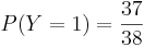 and
and 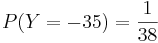 , as there are 38 numbers in total (0, 00, 1, 2, …, 36). The player may place a bet on any of these numbers, with a player success payoff of $35 (casino loss of $35) and a player loss of $1 (casino win of $1). Therefore, the casino expected return of the game is
 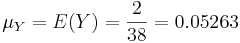 and the variance of the casino return is
 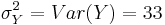 (σY = SD(Y) = 5.8) and the range of the return is [-35 : 1], for one game. The exact probability of interest may be computed by using Binomial Distribution. If the total casino return in 100 games is denoted by
  , then the expected casino return in 100 games is $5.26 and P(T>28)=P(X>k), where
  and k is the integer solution of the following dollar amount equation:
  . Therefore,
  . The last probability represents the exact solution and is computed using the SOCR Binomial Distribution applet. This exact calculation is numerically intractable for large sample-sizes (n>200), albeit approximations exist.
- Solution 2: One could use the CLT to find a very good approximation to this type of probabilities. For example, in the case above (n=100), we can estimate the probability of interest by
 Notice that this calculation is sample-size independent, and hence widely applicable, whereas the former exact probability calculation (Solution 1) is limited for small n. What caused the large discrepancy between the exact (
 ) and approximate (
 ) values of the probability of interest? This is an example where the usual rule of 30 measurements breaks, because of the skewed underlying Binomial distribution. Such limitations of the CLT even for large sample-sizes have been previously observed and reported for severely skewed distributions (Freedman, Pisani, & Purves, 1998). Here one would need much larger sample to get a reasonably good approximation using CLT. For example, if n=1,000, and we are looking for P(T > 100), then k=975, the exact probability is P(T > 100) = P(X > 975) = 0.4493287, and the CLT approximation is much closer:
- Solution 3: Finally, we show how one can use the SOCR CLT applet alone to completely empirically estimate the probability of interest, P(T>28), for n=100. The figure below demonstrates how we can manually construct the native probability mass function for the random variable Y (casino payoff of one roulette game). A simple linear transformation is needed to convert the values of Y to W (
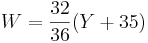 ), so that the range of the Y variable [-35 : 1] may be mapped to the default range of W, the native distribution [0 : 32]. Now, recalling the definitions above (for the n=100 case) we have that
  . The last equality is obtained by noticing that W will have approximately Normal(μ = 31.23332;σ2 = 0.488118952) distribution, with empirical mean and standard deviation obtained from row 3 in the table.

Additional Applications of the CLT are available here
- Back to SOCR CLT Activity
- SOCR Home page: http://www.socr.ucla.edu
- SOCR CLT Activity at MERLOT
- SOCR CLT Activity at CAUSEweb
- Dinov, ID, Christou, N, and Sanchez, J (2008) Central Limit Theorem: New SOCR Applet and Demonstration Activity. Journal of Statistics Education, Volume 16, Number 2.
Translate this page:
