SOCR EduMaterials AnalysisActivities SLR
From Socr
Contents |
SOCR Analysis Example on Simple Linear Regression
This SOCR Activity demonstrates the utilization of the SOCR Analyses package for statistical Computing. In particular, it shows how to use Simple Linear Regression and how to interpret the results.
Simple Linear Regression Background
Simple Linear Regression (SLR) is a class of statistical analysis models and procedures, which takes one independent variable and one dependent variable, both being quantitative, and models the relationship between them.
The model form is: y = intercept + slope * x + error, where x denotes the independent variable and y denotes the dependent variable. So it is linear. The error is assumed to follow a standard normal distribution.
The goal of the Simple Linear Regression computing procedure is to estimate the intercept and the slope, based on the data. Least Squares Fitting is used.
In this activity, the students can learn about:
- Reading results of Simple Linear Regression;
- Making interpretation of the slope and intercept;
- Observing and interpreting various data and resulting plots
- Scatter plots of the dependent vs. independent variables
- Diagnostic plots such as the Residual on Fit plot
- Normal QQ plot, etc.
SOCR Simple Linear Regression
Go to SOCR Analyses and select Simple Linear Regression from the drop-down list of SOCR analyses, in the left panel. There are three ways to enter data in the SOCR Simple Linear Regression applet:
- Click on the Example button on the top of the right panel.
- Generate random data by clicking on the Random Example button.
- Paste your own data from a spreadsheet into SOCR Simple Linear Regression data table.
SOCR Simple Linear Regression Example
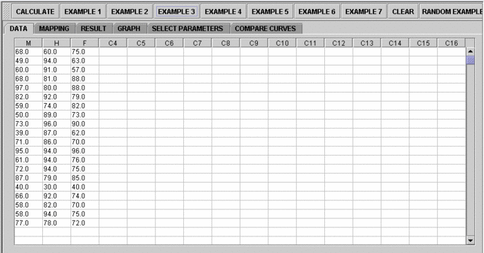
We will demonstrate SLR with some SOCR built-in examples. The first example (EXAMPLE 1) is based on the data taken from "An Introduction to Computational Statistics: Regression Analyses" by Robert Jennrich, Prentice Hall, 1995 (Page 4). The data describe exam and home scores of a class of students, where M stands for midterm, F for final, and H for homework.
- As you start the SOCR Analyses Applet, click on Simple Linear Regression from the combo box in the left panel. Here's what the screen should look like.
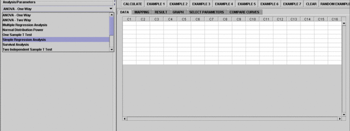
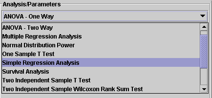
- The left part of the panel looks like this (make sure that the "Simple Linear Regression" is showing in the drop-down list of analyses, otherwise you won't be able to find the correct dataset and will not be able to reproduce the results!)
- in the SOCR SLR analysis, there are several SOCR built-in examples. In this activity, we'll be using Example 3. Click on the "Example 3" button and next, click on the "Data" button in the right panel. You should see the data displayed in two columns. There are three columns here, M, F and H.
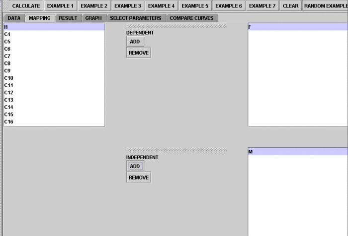
- Use column M as the regressor (that is, 'x', the independent variable) and column F as the response (that is, 'y', the dependent variable). So you can simply ignore the column H for this activity. To tell the computer which variables are assigned to be the regressor and response, we have to do a "Mapping." This is done by clicking on the "Mapping" button first to get to the Mapping Panel, and then map the variables. For this Simple Linear Regression activity, there are two places the variables can be mapped to. The top part says DEPENDENT that you'll need to map the dependent variable you want here. Just click on ADD under DEPENDENT and that will do it. If you change your mind, you can click on REMOVE. Similar for the INDEPENDENT variable. Once you get the screen to look like the screenshot below, you're done with the Mapping step. (Note that, since the columns C3 through C16 do not have data and they are not used, just ignore them.)
- After we do the "Mapping" to assign variables, now we use the computer to calculate the regression results -- click on the "Calculate" button. Then select the "Result" panel to see the output.
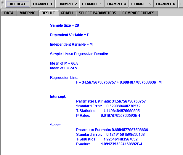
The text in the Result Panel summarizes the results of this simple linear regression analysis. The regression line is displayed. At this point, you can think about how the dependent variable changes, on average, in response to changes of the independent variable.
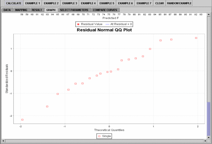
- If you'd like to see graphical component of this analysis, click on the "Graph" panel. You'll then see the graph panel that displays scatter plot, as well as diagnostic plots of "residual on fit", "Normal QQ" plots, etc. The plot titles indicate plot types.
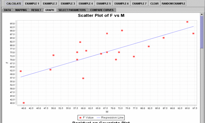
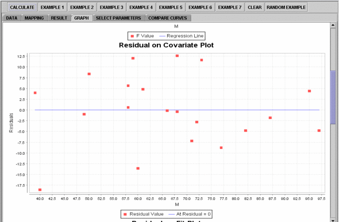
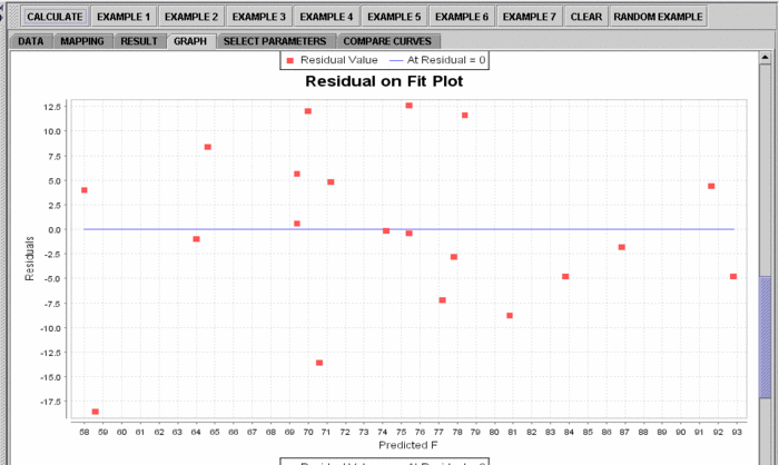
Note: If you happen to click on the "Clear" button in the middle of the procedure, all the data will be cleared out. Simply start over from step 1.
See also
Translate this page:
