AP Statistics Curriculum 2007 Distrib RV
From Socr
Contents |
General Advance-Placement (AP) Statistics Curriculum - Random Variables and Probability Distributions
Random Variables
A random variable is a function or a mapping from a sample space into the real numbers (most of the time). In other words, a random variable assigns real values to outcomes of experiments. This mapping is called random, as the output values of the mapping depend on the outcome of the experiment, which are indeed random. So, instead of studying the raw outcomes of experiments (e.g., define and compute probabilities), most of the time we study (or compute probabilities) on the corresponding random variables instead. The formal general definition of random variables may be found here.
Examples of Random Variables
- Die: In rolling a regular hexagonal die, the sample space is clearly and numerically well-defined and in this case the random variable is the identity function assigning to each face of the die the numerical value it represents. This the possible outcomes of the RV of this experiment are { 1, 2, 3, 4, 5, 6 }. You can see this explicit RV mapping in the SOCR Die Experiment.
- Coin: For a coin toss, a suitable space of possible outcomes is S={H, T} (for heads and tails). In this case these are not numerical values, so we can define a RV that maps these to numbers. For instance, we can define the RV
![X: S \longrightarrow [0, 1]](/socr/uploads/math/9/5/e/95e11d7a452f746b687a6e814bc71747.png) as:
as: 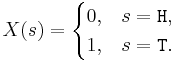 . You can see this explicit RV mapping of heads and tails to numbers in the SOCR Coin Experiment.
- Card: Suppose we draw a 5-card hand from a standard 52-card deck and we are interested in the probability that the hand contains at least one pair of cards with identical denomination. Then the sample space of this experiment is large - it should be difficult to list all possible outcomes. However, we can assign a random variable
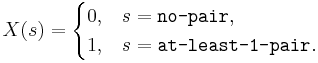 and try to compute the probability of P(X=1), the chance that the hand contains a pair. You can see this explicit RV mapping and the calculations of this probability at the SOCR Card Experiment.
Probability density/mass and (cumulative) distribution functions
- The probability density or probability mass function, for a continuous or discrete random variable, is the function defined by the probability:
- p(x) = P(allsS | X(s) = x), for each x.
- The cumulative distribution function (cdf) F(x) of any random variable X with probability mass or density function p(x) is defined by:
-
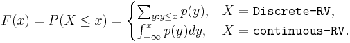 , for all x.
PDF Example
The Benford's Law states that the probability of the first digit (d) in a large number of integer observations ( ) is given by
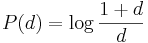 , for
, for 
Note that this probability definition determines a discrete probability (mass) distribution:
| d | 1 | 2 | 3 | 4 | 5 | 6 | 7 | 8 | 9 |
| P(d) | 0.301 | 0.176 | 0.125 | 0.097 | 0.079 | 0.067 | 0.058 | 0.051 | 0.046 |
The explanation of the Benford's Law may be summarized as follows: The distribution of the first digits must be independent of the measuring units used in observing/recording the integer measurements. For instance, this means that if we had observed people's heights in inches or centimeters (inches and centimeters are linearly dependent,  ), the distribution of the first digit must be unchanged. So, there are about three centimeters for each inch. Thus, the probability that the first digit of a heigth observation is 1in must be the same as the probability that the first digit of a heigth in centimeters starts with either 2 or 3 (with standard round off). Similarly, for observations of 2in, need to have their centimeter counterparts either 5cm or 6cm. Observations of 3in will correspond to 7 or 8 centimeters, etc. In other words, this distribution must be scale invariant.
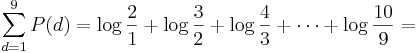
The only distribution that obeys this property is the one whose logarithm is uniformly distributed. In this case, the logarithms of the numbers are uniformly distributed --  =
=  is the same as the probability
  =
=  . Examples of such exponentially growing numerical measurements are incomes, stock prices and computational power.
How to Use RVs?
There are 3 important quantities that we are always interested in when we study random processes. Each of these may be phrased in terms of RVs, which simplifies their calculations.
- Probability Density Function (PDF): What is the probability of P(X = xo)? For instance, in the card example above, we may be interested in P(at least 1 pair) = P(X=1) = P(1 pair only) = 0.422569. Or in the die example, we may want to know P(Even number turns up) =
 .
.
- Cumulative Distribution Function (CDF): P(X < xo), for all xo. For instance, in the (fair) die example we have the following discrete density (mass) and cumulative distribution table:
| x | 1 | 2 | 3 | 4 | 5 | 6 |
| PDFP(X = x) | 1/6 | 1/6 | 1/6 | 1/6 | 1/6 | 1/6 |
CDF  | 1/6 | 2/6 | 3/6 | 4/6 | 5/6 | 1 |
- Mean/Expected Value: Most natural processes may be characterized, via probability distribution of an appropriate RV, in terms of a small number of parameters. These parameters simplify the practical interpretation of the process or phenomena we study. For example, it is often enough to know what the process (or RV) average value is. This is the concept of expected value (or mean) of a random variable, denoted E[X]. The expected value is the point of gravitational balance of the distribution of the RV.
Obviously, we may define a large number of RV for the same process. When are two RVs equivalent is dependent on the definition of equivalence?
The Web of Distributions
There are a large number of families of distributions and distribution classification schemes.
The most common way to describe the universe of distributions is to partition them into categories. For example, Continuous Distributions and Discrete Distributions; marginal and joint distributions; finitely and infinitely supported, etc.
SOCR Distribution applets and the SOCR Distribution activities illustrate how to use technology to compute probabilities for events arising from many different processes.
The image below shows some of the relations between commonly used distributions. Many of these relations will be explored later.

References
- SOCR Home page: http://www.socr.ucla.edu
Translate this page:
