AP Statistics Curriculum 2007 Estim S Mean
From Socr
Contents |
General Advance-Placement (AP) Statistics Curriculum - Estimating a Population Mean: Small Samples
Now we discuss estimation when the sample-sizes are small, typically < 30 observations. Naturally, the point estimates are less precise and the interval estimates produce wider intervals, compared to the case of large-samples.
Point Estimation of a Population Mean
The population mean may also be estimated by the sample average using a small sample. That is the sample average 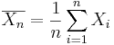 , constructed from a random sample of the process {
 }, which is an unbiased estimate of the population mean μ, if it exists! Note that the sample average may be susceptible to outliers.
Interval Estimation of a Population Mean
For small samples, interval estimations of the population means (or Confidence Intervals) are constructed as follows. Choose a confidence level (1 − α)100%, where α is small (e.g., 0.1, 0.05, 0.025, 0.01, 0.001, etc.). Then a (1 − α)100% confidence interval for μ is defined in terms of the T-distribution:
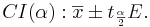
- The Error term, E, is defined as
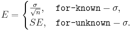
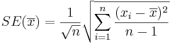
- The Standard Error of the estimate
 is obtained by replacing the unknown population standard deviation by the sample standard deviation:
 is the
Assumptions
To use the small-sample method for constructing a confidence interval for the population mean, we must have evidence that the data we observed and used for the point and interval estimates come from a distribution which is (approximately) Normal. If this assumption is violated, the interval estimate we compute may be significantly misrepresenting the real confidence interval!
Example
To parallel the example in the large sample case, we consider again the number of sentences per advertisement as a measure of readability for magazine advertisements. A random sample of the number of sentences found in 10 magazine advertisements is listed. Use this sample to find point estimate for the population mean μ (sample-mean=22.1, sample-variance=737.88 and sample-SD=27.16390579).
| 16 | 9 | 14 | 11 | 17 | 12 | 99 | 18 | 13 | 12 |
A confidence interval estimate of μ is a range of values used to estimate a population parameter (interval estimates are normally used more than point estimates because it is very unlikely that the sample mean would match exactly with the population mean) The interval estimate uses a margin of error about the point estimate.
Before you find an interval estimate, you should first determine how confident you want to be that your interval estimate contains the population mean.
- 80% confidence (0.80),
 , t(df=9) = 1.383
- 90% confidence (0.90),
 , t(df=9) = 1.833
- 95% confidence (0.95),
 , t(df=9) = 2.262
- 99% confidence (0.99),
 , t(df=9) = 3.250
Notice that for a fixed α, the t-critical values (for any degree-of-freedom) exceeds the corresponding normal z-critical values, which are used in the large-sample interval estimation. The SOCR Student's T distribution calculator may be used to obtain accurate critical and probability values for the T distribution.

Known Variance
Suppose that we know the variance for the number of sentences per advertisement example above is known to be 256 (so the population standard deviation is σ = 16).
- For , the 80%CI(μ) is constructed by:
![\overline{x}\pm 1.383{16\over \sqrt{10}}=22.1 \pm 1.28{16\over \sqrt{10}}=[15.10 ; 29.10]](/socr/uploads/math/e/1/0/e1081ddefb91f08893f7fee82b36d0f9.png)
- For , the 90%CI(μ) is constructed by:
![\overline{x}\pm 1.833{16\over \sqrt{10}}=22.1 \pm 1.833{16\over \sqrt{10}}=[12.83 ; 31.37]](/socr/uploads/math/8/6/b/86b29086b9601f64e74af59f2d301086.png)
- For , the 99%CI(μ) is constructed by:
![\overline{x}\pm 3.250{16\over \sqrt{10}}=22.1 \pm 3.250{16\over \sqrt{10}}=[5.66 ; 38.54]](/socr/uploads/math/4/0/7/4070206fb85f38ea4f86c455b4eba3a4.png)
Notice the increase of the CI's (directly related to the decrease of α) reflecting our choice for higher confidence.
Unknown Variance
Suppose that we do not know the variance for the number of sentences per advertisement but use the sample variance 737.88 as an estimate (so the sample standard deviation is  ).
).
- For , the 80%CI(μ) is constructed by:
![\overline{x}\pm 1.383{27.16390579\over \sqrt{10}}=22.1 \pm 1.383{27.16390579\over \sqrt{10}}=[10.22 ; 33.98]](/socr/uploads/math/2/9/5/29526e602f7993ef21bffa034b7416bf.png)
- For , the 90%CI(μ) is constructed by:
![\overline{x}\pm 1.833{27.16390579\over \sqrt{10}}=22.1 \pm 1.833{27.16390579\over \sqrt{10}}=[6.35 ; 37.85]](/socr/uploads/math/1/5/5/1551809ba9e0acb24af92d235aba6d52.png)
- For , the 99%CI(μ) is constructed by:
![\overline{x}\pm 3.250{27.16390579 \over \sqrt{10}}=22.1 \pm 3.250{27.16390579\over \sqrt{10}}=[-5.82 ; 50.02]](/socr/uploads/math/1/0/6/1060fbcb863b8873047a26931e983719.png)
Notice the increase of the CI's (directly related to the decrease of α) reflecting our choice for higher confidence.
Hands-on Activities
- See the SOCR Confidence Interval Experiment.
- Sample statistics, like the sample-mean and the sample-variance, may be easily obtained using SOCR Charts. The images below illustrate this functionality (based on the Bar-Chart and Index-Chart) using the 30 observations of the number of sentences per advertisement, reported above.


Problems
- SOCR Home page: http://www.socr.ucla.edu
Translate this page:
