AP Statistics Curriculum 2007 GLM Corr
From Socr
Contents |
General Advance-Placement (AP) Statistics Curriculum - Correlation
Many biomedical, social, engineering and science applications involve the analysis of relationships, if any, between two or more variables involved in the process of interest. We begin with the simplest of all situations where bivariate data (X and Y) are measured for a process and we are interested in determining the association, relation or an appropriate model for these observations (e.g., fitting a straight line to the pairs of (X,Y) data). If we are successful determining a relationship between X and Y, we can use this model to make predictions - i.e., given a value of X predict a corresponding Y response. Note that in this design, data consists of paired observations (X,Y) - for example, the height and weight of individuals.
Lines in 2D
There are 3 types of lines in 2D planes - Vertical Lines, Horizontal Lines and Oblique Lines. In general, the mathematical representation of lines in 2D is given by equations like aX + bY = c, most frequently expressed as Y = aX + b, provides the line is not vertical.
Recall that there is a one-to-one correspondence between any line in 2D and (linear) equations of the form
- If the line is vertical (X1 = X2): X = X1;
- If the line is horizontal (Y1 = Y2): Y = Y1;
- Otherwise (oblique line):
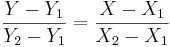 , (for
  and
and  )
)
where (X1,Y1) and (X2,Y2) are two points on the line of interest (2-distinct points in 2D determine a unique line).
- Try drawing the following lines manually and using this applet:
- Y=2X+1
- Y=-3X-5
The Correlation Coefficient
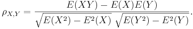
Correlation coefficient ( ) is a measure of linear association, or clustering around a line of multivariate data. The main relationship between two variables (X, Y) can be summarized by: (μX,σX), (μY,σY) and the correlation coefficient, denoted by ρ = ρ(X,Y) = R(X,Y).
- If ρ = 1, we have a perfect positive correlation (straight line relationship between the two variables)
- If ρ = 0, there is no correlation (random cloud scatter), i.e., no linear relation between X and Y.
- If ρ = − 1, there is a perfect negative correlation between the variables.
Computing ρ = R(X,Y)
The protocol for computing the correlation involves standardizing, multiplication and averaging.
- In general, for any random variable:
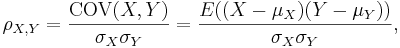
where E is the expected value operator and COV means covariance.
Since μX = E(X), 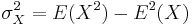 and similarly for Y, we may also write
- Sample correlation - we only have sampled data - we replace the (unknown) expectations and standard deviations by their sample analogues (sample-mean and sample-standard deviation) to compute the sample correlation:
- Suppose {
 } and {
 } are bivariate observations of the same process and (μX,σX) and (μY,σY) are the means and standard deviations for the X and Y measurements, respectively.
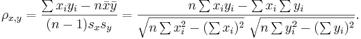
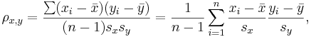
where  and
and  are the sample means of X and Y , sx and sy are the sample standard deviations of X and Y and the sum is from i = 1 to n. We may rewrite this as
- Note: The correlation is defined only if both of the standard deviations are finite and are nonzero. It is a corollary of the Cauchy-Schwarz inequality that the correlation is always bounded .
Examples
Human weight and height
Suppose we took only 6 of the over 25,000 observations of human weight and height included in this SOCR Dataset.
| Subject Index | Height(xi) in cm | Weight (yi) in kg |  |  |  |  | 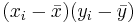
|
| 1 | 167 | 60 | 6 | 4.67 | 36 | 21,82 | 28.02 |
| 2 | 170 | 64 | 9 | 8.67 | 81 | 75.17 | 78.03 |
| 3 | 160 | 57 | -1 | 1.67 | 1 | 2.79 | -1.67 |
| 4 | 152 | 46 | -9 | -9.33 | 81 | 87.05 | 83.97 |
| 5 | 157 | 55 | -4 | -0.33 | 16 | 0.11 | 1.32 |
| 6 | 160 | 50 | -1 | -5.33 | 1 | 28.41 | 5.33 |
| Total | 966 | 332 | 0 | 0 | 216 | 215.33 | 195.0 |
We can easily now compute by hand 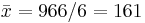 (cm),
(cm), 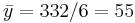 (kg),
(kg), 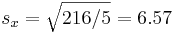 and
and 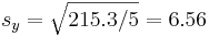 .
.
Therefore, 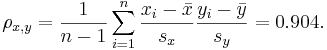
Of course, these calculations become difficult for more than a few paired observations and that is why we use the Simple Linear Regression in SOCR Analyses to compute the correlation and other linear associations in the bivariate case. The image below shows the calculations for the same data shown above in SOCR.

Use the Simple Linear Regression to compute the correlation between the height and weight in the first 200 measurements in the human weight and height included in this SOCR Dataset.
Hot-dogs dataset
Use the Simple Linear Regression to compute the correlation between the calories and sodium in the Hot-dogs dataset.
Airfare Example
Suppose we have the following bivariate X={airfare} and Y={distance traveled from Baltimore, MD} measurements:
| Destination | Distance | Airfare |
| Atlanta | 576 | 178 |
| Boston | 370 | 138 |
| Chicago | 612 | 94 |
| Dallas | 1216 | 278 |
| Detroit | 409 | 158 |
| Denver | 1502 | 258 |
| Miami | 946 | 198 |
| New_Orleans | 998 | 188 |
| New_York | 189 | 98 |
| Orlando | 787 | 179 |
| Pittsburgh | 210 | 138 |
| St._Louis | 737 | 98 |
Use the Simple Linear Regression to find the correlation between ticket fare and the distance traveled by passengers. Explain your findings.
Properties of the Correlation Coefficient
- The correlation is associative operation: ρ(X,Y) = ρ(Y,X)
- The correlation is (almost) linearly invariant:
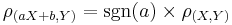 . If a > 0, then ρ(aX + b,Y) = ρ(X,Y). If a < 0, then ρ(aX + b,Y) = − ρ(X,Y).
- A trivial correlation, ρX,Y = 0 only implies that there is no linear relation between X and Y, but there may be other relations (e.g., quadratic). Therefore, statistical independence of X and Y does imply that ρX,Y = 0. However the converse is false, ρX,Y = 0 does not imply independence!
- A high correlation between X and Y does not imply causality (i.e., does not mean that one of the variables causes the observed behavior in the other. For example, consider X={math scores} and Y={shoe size) for all K-12 students. X and Y are very highly positively correlated, yet higher shoe sizes do not imply better math skills.
- The complete properties of the Correlation coefficients may be found here.
Statistical inference on correlation coefficients
- Testing a single correlation coefficient (Ho:r = ρ vs.
 ):
):
- There is a simple statistical test for the correlation coefficient. Suppose we want to test if the correlation between X and Y is equal to rho. If our bivariate sample is of size N and the observed sample correlation is r, then the test statistics is:
-
 , which has T-distribution with df=N—2.
-
- Comparing two correlation coefficients: The Fisher's transformation provides a mechanism to test for comparing two correlation coefficients using Normal distribution. Suppose we have 2 independent paired samples
 and
and  , and the r1=corr(X,Y) and r2=corr(U,V) and we are testing Ho:r1 = r2 vs.
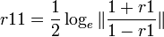
  . The Fisher's transformation for the 2 correlations is defined by:
-
- Transforming the two correlation coefficients separately yields:
 , and
, and
- Then the test statistics
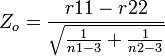 is Standard Normally distributed.
- Example: The following dataset represents the brain volume (predictors) measurements and ages (responses) for 2 cohorts of subjects (group1 and group2):
| Group1 | Age1 | Volume1 | Group2 | Age2 | Volume2 |
|---|---|---|---|---|---|
| 1 | 64 | 0.245517 | 2 | 30 | 0.29165 |
| 1 | 30 | 0.308443 | 2 | 38 | 0.297111 |
| 1 | 37 | 0.294692 | 2 | 46 | 0.275401 |
| 1 | 62 | 0.279998 | 2 | 55 | 0.284923 |
| 1 | 59 | 0.256802 | 2 | 37 | 0.287809 |
| 1 | 51 | 0.293875 | 2 | 41 | 0.291287 |
| 1 | 52 | 0.28895 | 2 | 57 | 0.26833 |
| 1 | 59 | 0.29262 | 2 | 69 | 0.268375 |
| 1 | 33 | 0.283666 | 2 | 69 | 0.253352 |
| 1 | 47 | 0.27458 | 2 | 41 | 0.292208 |
| 1 | 62 | 0.27269 | 2 | 60 | 0.276306 |
| 1 | 58 | 0.269609 | 2 | 59 | 0.27905 |
| 1 | 55 | 0.277243 | 2 | 50 | 0.262916 |
| 1 | 61 | 0.236264 | 2 | 58 | 0.290697 |
| 1 | 70 | 0.218015 | 2 | 58 | 0.269361 |
| 1 | 38 | 0.287205 | 2 | 61 | 0.268247 |
| 1 | 41 | 0.307387 | 2 | 57 | 0.294204 |
| 1 | 40 | 0.271063 | 2 | 50 | 0.292699 |
| 1 | 25 | 0.307688 | 2 | 38 | 0.273969 |
| 1 | 70 | 0.237811 | 2 | 57 | 0.29049 |
| 1 | 49 | 0.293371 | 2 | 64 | 0.286564 |
| 1 | 56 | 0.252592 | 2 | 71 | 0.257386 |
| 1 | 56 | 0.251349 | 2 | 34 | 0.314958 |
| 1 | 40 | 0.29616 | 2 | 53 | 0.298022 |
| 1 | 50 | 0.249596 | 2 | 53 | 0.269229 |
| 1 | 55 | 0.282721 | 2 | 25 | 0.270634 |
| 1 | 69 | 0.247565 | 2 | 61 | 0.266905 |
- We have 2 independent groups (Group1 and Group2) and X=Volume1 and Y=Age1; U=Volume2 and V=Age2, n1=27, n2=27. We can also compute the 2 correlation coefficients:
- r1 = corr(X,Y) = − 0.75339, and
- r2 = corr(U,V) = − 0.49491
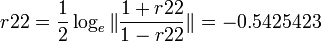
- Using the Fisher's transformation we obtain:
 , and
, and
- And thus,
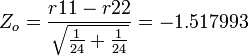 and a corresponding p-value = 0.064508.
Problems
References
- SOCR Analyses / Simple Linear Regression Applet
- Correlation/Regression Experiment
- Interactive Correlation/Regression Game
- SOCR Home page: http://www.socr.ucla.edu
Translate this page:
