AP Statistics Curriculum 2007 Infer BiVar
From Socr
(→Comparing Two Variances (\sigma_1^2 = \sigma_2^2?)) |
|||
| Line 9: | Line 9: | ||
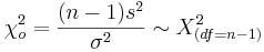
: <math>\chi_o^2 = {(n-1)s^2 \over \sigma^2} \sim \Chi_{(df=n-1)}^2</math> | : <math>\chi_o^2 = {(n-1)s^2 \over \sigma^2} \sim \Chi_{(df=n-1)}^2</math> | ||
| - | ===Comparing Two Variances ( | + | ===Comparing Two Variances (\(\sigma_1^2 = \sigma_2^2\)?)=== |
Suppose we study two populations which are approximately Normally distributed, and we take a random sample from each population, {<math>X_1, X_2, X_3, \cdots, X_n</math>} and {<math>Y_1, Y_2, Y_3, \cdots, Y_k</math>}. Recall that <math>{(n-1) s_1^2 \over \sigma_1^2}</math> and <math>{(n-1) s_2^2 \over \sigma_2^2}</math> have <math>\Chi^2_{(df=n - 1)}</math> and <math>\Chi^2_{(df=k - 1)}</math> distributions. We are interested in assessing <math>H_o: \sigma_1^2 = \sigma_2^2</math> vs. <math>H_1: \sigma_1^2 \not= \sigma_2^2</math>, where <math>s_1</math> and <math>\sigma_1</math>, and <math>s_2</math> and <math>\sigma_2</math> and the sample and the population standard deviations for the two populations/samples, respectively. | Suppose we study two populations which are approximately Normally distributed, and we take a random sample from each population, {<math>X_1, X_2, X_3, \cdots, X_n</math>} and {<math>Y_1, Y_2, Y_3, \cdots, Y_k</math>}. Recall that <math>{(n-1) s_1^2 \over \sigma_1^2}</math> and <math>{(n-1) s_2^2 \over \sigma_2^2}</math> have <math>\Chi^2_{(df=n - 1)}</math> and <math>\Chi^2_{(df=k - 1)}</math> distributions. We are interested in assessing <math>H_o: \sigma_1^2 = \sigma_2^2</math> vs. <math>H_1: \sigma_1^2 \not= \sigma_2^2</math>, where <math>s_1</math> and <math>\sigma_1</math>, and <math>s_2</math> and <math>\sigma_2</math> and the sample and the population standard deviations for the two populations/samples, respectively. | ||
Current revision as of 14:44, 14 February 2014
Contents |
General Advance-Placement (AP) Statistics Curriculum - Comparing Two Variances
In the section on inference about the variance and the standard deviation, we already learned how to do inference on either of these two population parameters. Now we discuss the comparison of the variances (or standard deviations) using data randomly sampled from two different populations.
Background
Recall that the sample-variance (s2) is an unbiased point estimate for the population variance σ2, and similarly, the sample-standard-deviation (s) is a point estimate for the population-standard-deviation σ.
The sample-variance is roughly Chi-square distributed:
Comparing Two Variances (\(\sigma_1^2 = \sigma_2^2\)?)
Suppose we study two populations which are approximately Normally distributed, and we take a random sample from each population, {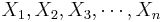 } and {
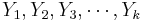 }. Recall that
  and
and  have
have  and
and  distributions. We are interested in assessing
 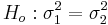 vs.
vs.  , where s1 and σ1, and s2 and σ2 and the sample and the population standard deviations for the two populations/samples, respectively.
Notice that the Chi-Square Distribution is not symmetric (it is positively skewed). You can visualize the Chi-Square distribution and compute all critical values either using the SOCR Chi-Square Distribution or using the SOCR Chi-Square Distribution Calculator.
The Fisher's F Distribution, and the corresponding F-test, is used to test if the variances of two populations are equal. Depending on the alternative hypothesis, we can use either a two-tailed test or a one-tailed test. The two-tailed version tests against an alternative that the standard deviations are not equal (). The one-tailed version only tests in one direction ( or
or  ). The choice is determined by the study design before any data is analyzed. For example, if a modification to an existent medical treatment is proposed, we may only be interested in knowing if the new treatment is more consistent and less variable than the established medical intervention.
- Test Statistic:

The farther away this ratio is from 1, the stronger the evidence for unequal population variances.
- Inference: Suppose we test at significance level α = 0.05. Then the hypothesis that the two standard deviations are equal is rejected if the test statistics is outside this interval
- : If Fo > F(α,df1 = n1 − 1,df2 = n2 − 1)
- : If Fo < F(1 − α,df1 = n1 − 1,df2 = n2 − 1)
- : If either Fo < F(1 − α / 2,df1 = n1 − 1,df2 = n2 − 1) or Fo > F(α / 2,df1 = n1 − 1,df2 = n2 − 1),
where F(α,df1 = n1 − 1,df2 = n2 − 1) is the critical value of the F distribution with degrees of freedom for the numerator and denominator, df1 = n1 − 1,df2 = n2 − 1, respectively.
In the image below, the left and right critical regions are white with F(α,df1 = n1 − 1,df2 = n2 − 1) and F(1 − α,df1 = n1 − 1,df2 = n2 − 1) representing the lower and upper, respectively, critical values. In this example of F(df1 = 12,df2 = 15), the left and right critical values at α / 2 = 0.025 are F(α / 2 = 0.025,df1 = 9,df2 = 14) = 0.314744 and F(1 − α / 2 = 0.975,df1 = 9,df2 = 14) = 2.96327, respectively.

Comparing Two Standard Deviations (σ1 = σ2?)
To make inference on whether the standard deviations of two populations are equal, we calculate the sample variances and apply the inference on the ratio of the sample variance using the F-test, as described above.
Hands-on activities
- Formulate appropriate hypotheses and assess the significance of the evidence to reject the null hypothesis that the variances of the two populations, where the following data come from, are distinct. Assume the observations below represent random samples (of sizes 6 and 10) from two Normally distributed populations of liquid content (in fluid ounces) of beverage cans. Use (α = 0.1).
| Sample from Population 1 | 14.816 | 14.863 | 14.814 | 14.998 | 14.965 | 14.824 | ||||
| Sample from Population 2 | 14.884 | 14.838 | 14.916 | 15.021 | 14.874 | 14.856 | 14.860 | 14.772 | 14.980 | 14.919 |
- Hypotheses: Ho:σ1 = σ2 vs.
 .
.
- Get the sample statistics from SOCR Charts (e.g., Index Plot);
| Sample Mean | Sample SD | Sample Variance | |
| Sample 1 | 14.88 | 0.081272382 | 0.0066052 |
| Sample 2 | 14.892 | 0.071269442 | 0.005079333 |

- Identify the degrees of freedom (df1 = 6 − 1 = 5 and df2 = 10 − 1 = 9).
- Test Statistics:
- Significance Inference: P-value=
 . This p-value does not indicate strong evidence in the data to reject the null hypothesis. That is, the data does not have power to discriminate between the population variances of the two populations based on these (small) samples.

More examples
- Use the hot-dogs dataset to formulate and test hypotheses about the difference of the population standard deviations of sodium between the poultry and the meet based hot-dogs. Repeat this with variances of calories between the beef and meet based hot-dogs.
See also
Fligner-Killeen non-parametric test for variance homogeneity.
References
- SOCR Home page: http://www.socr.ucla.edu
Translate this page:
