SOCR EduMaterials Activities ProportionEstimateExperiment
From Socr
Contents |
Proportion Estimate Experiment
Description
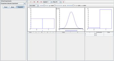
The experiment is to select a random sample of size n from the Bernoulli distribution with parameter p, and then to construct and approximate confidence interval for p at a specified confidence level. The true value of p can be varied with a scroll bar. The density of the Bernoulli distribution and the value of p are shown in blue in the first graph.
The confidence level can be selected from a list box, as well as the type of interval – two sided, upper bound, or lower bound. The interval is constructed using quantities from the standard normal distribution. The standard normal density and the critical values are shown in blue in the second graph.
Variables L and R denote the left and right endpoints of the confidence interval and I indicates the event that the confidence interval contains p. The theoretical density of I is shown in blue in the third graph.
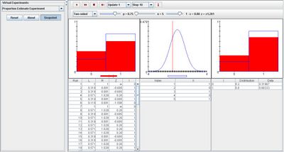
On each update, the sample density and the confidence interval are shown in red in the first graph, and the computed standard score is shown in red in the second graph. Note that the confidence interval contains p in the first graph if and only if the standard score falls between the critical values in the second graph. The third graph shows the proportion of successes and failures in red. The first table gives the sample values; the second table records L, R, the standard score Z, and I. Finally, the third table gives the theoretical and empirical densities of I.
Goal
The purpose is to provide a simulation that provides data from the Bernoulli distribution that allows others to develop a better understanding of confidence intervals numerically and graphically. It will give them the advantage to develop their own generalizations regarding proportion estimates and theoretical tests.
Experiment
Go to the SOCR Experiment [[1]] and select the Proportion Estimate Experiment from the drop-down list of experiments on the top left. The image below shows the initial view of this experiment:

When pressing the play button, one trial will be executed and recorded in the distribution table below. The fast forward button symbolizes the nth number of trials to be executed each time. The stop button ceases any activity and is helpful when the experimenter chooses “continuous,” indicating an infinite number of events. The fourth button will reset the entire experiment, deleting all previous information and data collected.
The “update” scroll indicates nth number of trials (1, 10, 100, or 1000) performed when selecting the fast forward button and the “stop” scroll indicates the maximum number of trials in the experiment.
Initially, the experiment is set to two-sided in the list box. When varying parameter p, note that the distribution in the first graph changes; increasing p will increase the probability for value 1 and decreasing the probability for value 0, and decreasing p will increase probability for 0 and decrease probability for 1. For the furthest scroll bar that represents 1 – alpha, increasing this parameter will increase the probability value of 1 and decrease the probability value of 0 in the far right graph. It will also increase the spread of the second graph, in which it is centered at the middle. The image below demonstrates these properties:

For the lower and upper bound selections in the list box, varying parameter p gives the same changes in the left and right graphs. The only difference is when increasing 1 – alpha, the varying spread will either be centered in the lower bound or upper bound, depending on the selection box. The image below illustrates this event when selecting upper bound:

Note, whenever varying 1 – alpha, the data is unlikely to fall in the outer tails of the middle graph.
Applications
The Proportion Estimate Experiment is a simple simulation that demonstrates the differences of confidence intervals and theoretical estimates. It may be used in many different types of events such as:
Suppose the probability of catching fish has normal distribution, but a fisherman suggests that the probability of catching fish is actually very small. By obtaining enough information, the fisherman may be able to use this simulation to demonstrate his theory analytically and graphically.
Translate this page:
