SOCR BivariateNormal JS Activity
From Socr
Contents |
SOCR Educational Materials - Activities - SOCR Bivariate Normal Distribution Activity
This activity represents a 3D rendering of the Bivariate Normal Distribution. It is implemented in HTML5/JavaScript and should be portable on any computer, operating system and web-browser.
Goals
The aims of this activity are to:
- Provide a visualization tool for better understanding of the bivariate normal distribution.
- Clarify the definitions and interplay between marginal, conditional and joint probability distributions (in the bivariate Normal case).
- Learn how to calculate Normal marginal, conditional and joint probabilities.
- Show how correlation influences the distribution of two normally-distributed variables. Demonstrate that when X and Y have joint bivariate normal distribution with zero correlation, then X and Y must be independent.
- Build a framework for generalizing the univariate normal distribution to higher dimensions.
Background
- In general, when X and Y are jointly continuous random variables with a joint density \(ƒ_{X,Y}(x,y)\), if A and B (non-trivial) are subsets of the ranges of X and Y (e.g., intervals), then:
- \( P(X \in A \mid Y \in B) = \frac{\int_{y\in B}\int_{x\in A} f_{X,Y}(x,y)\,dx\,dy}{\int_{y\in B}\int_{x\in\Omega} f_{X,Y}(x,y)\,dx\,dy}. \)
- In the special case where B={y0}, representing a single point, the conditional probability is:
- \( P(X \in A \mid Y = y_0) = \frac{\int_{x\in A} f_{X,Y}(x,y_0)\,dx}{\int_{x\in\Omega} f_{X,Y}(x,y_0)\,dx}\). If the set (range) A is trivial, then the conditional probability is zero.
- Suppose that X has normal distribution, the conditional mean of X given \(Y=y_o\), \(E(X|Y=y_o)\), is linear in Y, and the conditional variance of X given \(y_o\), \(Var(X|y_0)\), is constant. Then, the conditional probability distribution of X given Y = \(y_0\), \(f_{X|Y=y_o}\), is given by:
- \( f_{X|y_o} \sim N \left ( \mu_{X|y_o} = \mu_X +\rho \frac{\sigma_X}{\sigma_Y}(y_o-\mu_Y), \sigma_{X|y_o}^2 = \sigma_X^2(1-\rho^2) \right) \), where
- \( X \sim N (\mu_X, \sigma_X^2) \),
- \( E(Y)=\mu_Y\), and \(VAR(Y)=E(Y^2)-\mu_Y^2 = \sigma_Y^2 \), but this does not necessarily require that Y is normally distributed itself!
- \( \rho = Corr(X,Y)\) is the correlation between X and Y.
- This expression of the density assumes that the conditional mean of X given \(y_o\) is linear in y and the conditional variance of X given \(y_o\) is constant.
- The above does not make assumption about the distribution of Y. Now assume Y is also normally distributed with \( Y \sim N (\mu_Y, \sigma_Y^2) \). We have 3 important observations:
- 1. The density of Y is:
- \( f_Y = \frac{1}{\sigma_Y \sqrt{2\pi}} e^{-\frac{(y-\mu_y)^2}{2\sigma_Y^2}} \),
- 2. The conditional distribution of \(X\) given \(Y = y_o\) is:
- \( g_{X|Y}(x|y) = \frac{1}{\sigma_{X|Y} \sqrt{2\pi}} e^{-\frac{(x-\mu_{X|Y})^2}{2\sigma_{X|Y}^2}} \),
- \( = \frac{1}{\sigma_X\sqrt{1-\rho^2} \sqrt{2\pi}} e^{-\frac{(x-\mu_X-\rho\frac{\sigma_X}{\sigma_Y}(Y-\mu_Y))^2}{2\sigma_X^2(1-\rho^2)}} \)
- \( g_{X|Y}(x|y) = \frac{1}{\sigma_{X|Y} \sqrt{2\pi}} e^{-\frac{(x-\mu_{X|Y})^2}{2\sigma_{X|Y}^2}} \),
- 3. The joint probability density function of \(X\) and \(Y\) is:
- \( f_{X,Y}(x,y) = g_{X|Y}(x|y)f_Y(y) = \frac{1}{\sigma_X\sigma_Y 2\pi\sqrt{1-\rho^2}} e^{-q(x,y)} \), where
- \( q(x,y) = \frac{1}{2} \frac{1}{1-\rho^2} \left ( \left ( \frac{x-\mu_X}{\sigma_X} \right )^2 -2\rho\frac{x-\mu_X}{\sigma_X}\frac{y-\mu_Y}{\sigma_Y} +\left ( \frac{y-\mu_Y}{\sigma_Y} \right )^2 \right ) \).
- \( f_{X,Y}(x,y) = g_{X|Y}(x|y)f_Y(y) = \frac{1}{\sigma_X\sigma_Y 2\pi\sqrt{1-\rho^2}} e^{-q(x,y)} \), where
Requirements & usability
A modern web-browser with HTML and JavaScript support is required (mobile devices should be fine). The 3D view of the bivariate Normal distribution requires WebGL support, however this is not absolutely necessary. If you toggle off the "Use WebGL" check-box in the Settings panel you can view the 3D grid/mesh representation of the 2D Normal/Gaussian distribution without WebGL.
- Go to the SOCR Bivariate Normal Distribution Webapp.
- Use the Settings to initialize the web-app.
- In the Control panel:
- Select the appropriate bivariate limits for the X and Y variables.
- Choose desired Marginal or Conditional probability function.
- 1D Normal Distribution graph will be shown to the right.
- You can rotate and manipulate the bivariate normal distribution in 3D by clicking and dragging on the graph below.
- Probability Results are reported in the bottom text area.
Learning Activity: Human Height and Weight
In this interactive activity, we will use Height vs. Weight data for a random sample of 200 adolescents.
Parameter Estimation
Use the SOCR Modeler & the modeler activity to estimate the mean and standard deviation (SD) of the Height and Weight variables. Also, investigate the distribution of the two variables. By looking at the distributions of the two variables, we can conclude that Height and Weight roughly follow a normal distribution.
- For Height variable, the distribution is roughly normal.

The estimate of the mean of height is 67.95, and the estimate of the standard deviation for height is 1.94.

- For Weight variable, the distribution is slightly skewed, but still resembles normal.

The estimate of the mean of weight is 127.22, and the estimate of the standard deviation for weight is 11.96.

- To estimate the correlation between height and weight we use the SOCR SLR applet, see the corresponding activity. Map height as the dependent variable and weight as the independent variable. Click “Calculate” to obtain the summary statistics. The correlation between Height and Weight is 0.557.

Marginal distribution
Now, plug these 5 estimated quantities into the SOCR Bivariate Normal Webapp. Look at the marginal distribution of height and weight. How do they compare to their histograms from the SOCR Modeler?

When looking at marginal distributions, we disregard the variables we do not care about. For the bivariate normal case, the marginal distribution of a single variable is the distribution of the variable itself.
- Marginal of Weight: The histogram for weight spanned an interval of 92 to 165 pounds. The marginal distribution of weight spans an interval of 79 to 175 pounds. This interval is larger because the distribution of weight is not perfectly normal. Still, it does a good job of capturing the overall shape of weight.

- Marginal of Height: In the histogram of height, the data spanned an interval of 62 to 75 inches. The marginal distribution of height from the BVN applet spans an interval of 60 to 75 inches. This is largely because Height is normally distributed and can be approximated by a normal distribution.

Joint Probability
What is the probability of a randomly selected adolescent being between 65 and 70 inches tall and weighing between 120 and 140 pounds? To answer this question, change the Bivariate Normal limits to 120 < X < 140 and 65 < Y < 70. Here is the distribution of the probability set:

Look at the Probability Results. The probability of a randomly selected adolescent being between 65 and 70 inches tall and weighing between 120 and 140 pounds is 0.4894.

Marginal Probability
Disregarding weight, what is the probability that a randomly selected adolescent will be between 65 and 70 inches? Look at the marginal distribution of height. The probability that an adolescent will be between 65 and 70 inches is 0.799.

Conditional Probability
Given an adolescent is of average height, what is the probability the adolescent weighs between 120 and 140 pounds? This question requires the conditional distribution of weight. First, we need to change the Bivariate Limits so height only includes the average height: 67.95.


Given an adolescent is of average height, the probability that the adolescent weighs between 120 and 140 pounds is 0.669.
Practice experiments
Height vs. Weight
Use the SOCR Height vs. Weight dataset.
- Motivation: Human heights and weights are correlated, how do the marginal parameters for each of the height and weight distributions, and their correlation, affect the joint and conditional probabilities?
- Use the SOCR Modeler and the SOCR Modeler activity to estimate the mean and standard deviation of each of the 2 variables (people's heights and weights).
- Use the SOCR Simple Linear Regression applet, and the corresponding activity, to estimate the correlation (\(\rho=Corr(Height, Weight)\)).
- Use these 5 estimated quantities to apply the SOCR BVN Webapp to compute various probabilities of interest (phrased in the context of the data itself!):
- Marginal (e.g., \(P(Weight<150)\)),
- Conditional (e.g., \(P(Weight<150 \vert Height<63)\)),
- Joint (e.g., \(P(Height>60 \cap Weight<160)\)).
Inflation vs. HPI
Use the SOCR Inflation vs. Housing Price Index (HPI) dataset.
- Motivation: There are intricate associations between different social and economic factors like inflation, interest rate, consumer price index and housing price index. We can explore how marginal parameters for each of the Inflation and HPI distributions, and their correlation, affect their joint and conditional probabilities?
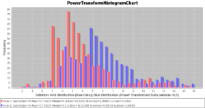
- Caution: This example is a little different from the human height and weight experiment above. In general, HPI and inflation may not follow normal distributions and may be skewed. Use the SOCR Histogram Chart to plot their distributions. Can the Bivariate Normal Distribution be used as an approximate model of the bivariate relation/probabilities of inflation and HPI? How about if we apply a data transformation? For example, the figure below shows the result of applying a square-root-transformation to the inflation variable (\(\lambda=0.5\)). The blue distribution of the transformed data is closer to Normal (note the skewness and kurtosis) compared to the red histogram of the raw inflation values.
- Use the SOCR Modeler and the SOCR Modeler activity to estimate the mean and standard deviation of each of the 2 variables (inflation and HPI).
- Use the SOCR Simple Linear Regression applet, and the corresponding activity, to estimate the correlation (\(\rho=Corr(Inflation,HPI)\)).
- Use these 5 estimated quantities to apply the SOCR BVN Webapp to compute various probabilities of interest (phrased in the context of the data itself!):
- Marginal (e.g., \(P(Inflation<2.0)\)),
- Conditional (e.g., \(P(Inflation>5.0 \vert HPI <108)\)),
- Joint (e.g., \(P(Inflation>4.0 \cap HPI<110)\)).

References
- See the EBook Multivariate Normal Distribution Chapter
- See also the SOCR 2D Point Segmentation using EM Mixture modeling activity
- Dinov, ID, Christou, N and Sanchez, J. (2008) Central Limit Theorem: New SOCR Applet and Demonstration Activity, Journal of Statistics Education, Volume 16, Number 2.
Translate this page:
